Cryptocurrencies - Python Data Analysis

Bitcoin was launched in 2008 since then many similiar currencies based on blockchain technology have emerged. The so called cryptocurrencies. Many of them are already extremly valuable e.g. Bitcoin, Bitcoin Cash or Etherum. However, investing in cryptocurrencies is extremly risky. The market is exceptionally volatile and any money you put in might disappear. As you can see at current events (Musk investing in Bitcoin etc.) the market is extremly volatile to this date. This data set was published on 6th December 2017 using the coinmarketcap API. (Source: coinmarketcap.com)

# imports
import pandas as pd
import matplotlib.pyplot as plt

# Setting aesthetics
plt.style.use('fivethirtyeight')

# Read in Data
filename= "/Users/max/Documents/My_Website/Data_Analysis_Projects/Exploring the Bitcoin Cryptocurrency Market/datasets/coinmarketcap_06122017.csv"
dec6 = pd.read_csv(filename)

# Subset 'id', 'market_cap_usd' columns
cols= ['id', 'market_cap_usd']
market_cap_raw = dec6[cols]

# Counting the number of values
market_cap_raw.count()

## id                1326
## market_cap_usd    1031
## dtype: int64

Simple Data Cleaning

The counts differ because some cryptocurrencies listed in coinmarketcap.com have no known market capitalization, this is represented by NaN in the data. The NaNs are not counted by count(). These cryptocurrencies are of little interest in this analysis, so they are safe to remove.

# Removing Coins withou market cap
cap = market_cap_raw.query('market_cap_usd > 0')

# Counting the number of values again --> match
cap.count()

## id                1031
## market_cap_usd    1031
## dtype: int64

Market capitalization of top 10 cryptocurrencies

Bitcoin is was and is dominant in market capitalization, but many other are competing for the No.1 spot . The following plot shows the top 10 coins as a barplot. (Data from 2017!)

#Variables
title = 'Top 10 market capitalization'
ylabel = '% of total cap'

# Selecting top 10
cap10 = cap[:10].set_index('id')

# Calculating market_cap_perc
cap10 = cap10.assign(market_cap_perc = lambda x: (x.market_cap_usd / cap.market_cap_usd.sum())*100)

# Plotting 
ax = cap10.market_cap_perc.plot.bar(title=title, color= "darkorange")

# Annotations
ax.set_ylabel(ylabel);
ax.set_xlabel("")
plt.tight_layout()
plt.show()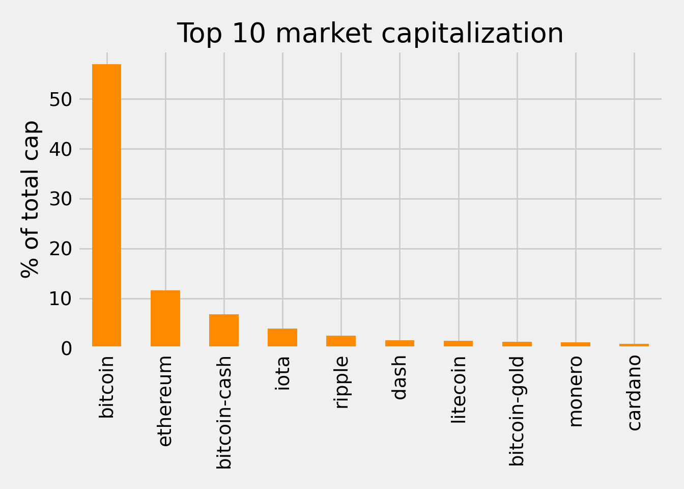

Volatility in cryptocurrencies

The cryptocurrencies market has been spectacularly volatile to this day. The next chunk shows the 24 hours and 7 days percentage change, which we already have available.

# Subset id, percent_change_24h and percent_change_7d columns
cols= ['id', 'percent_change_24h', 'percent_change_7d']
volatility = dec6[cols]

# Set index to 'id' 
volatility = volatility.set_index('id').dropna()

# Sorting by percent_change_24h in ascending order
volatility = volatility.sort_values(by= "percent_change_24h", ascending= True)

# Check
print(volatility.head())

##                percent_change_24h  percent_change_7d
## id                                                  
## flappycoin                 -95.85             -96.61
## credence-coin              -94.22             -95.31
## coupecoin                  -93.93             -61.24
## tyrocoin                   -79.02             -87.43
## petrodollar                -76.55             542.96

Well, we can already see that things are a bit crazy It seems you can lose a lot of money quickly on cryptocurrencies . The next plot shows the top 10 biggest gainers and top 10 losers in market capitalization. For that I defined a function which is shown in the enxt chunk.

# function with 2 parameters

def top10_subplot(volatility_series, title):
    
    # creating subplots
    fig, axes = plt.subplots(nrows=1, ncols=2, figsize=(10, 6))
    
    # Plotting barchart
    
    ax = volatility_series[:10].plot.bar(color="darkred", ax=axes[0],xlabel= "Coins")
    
    # Annotations
    fig.suptitle(title)
    ax.set_ylabel('% change')
    # top 10 winners 
    ax = volatility_series[-10:].plot.bar(color="darkblue", ax=axes[1],xlabel= "Coins")
    return fig, ax

TITLE = "24 hours top losers and winners"

# Calling the function above with the volatility.percent_change_24h series
# and title DTITLE 
fig, ax = top10_subplot(volatility.percent_change_24h, TITLE)
plt.tight_layout()
plt.show()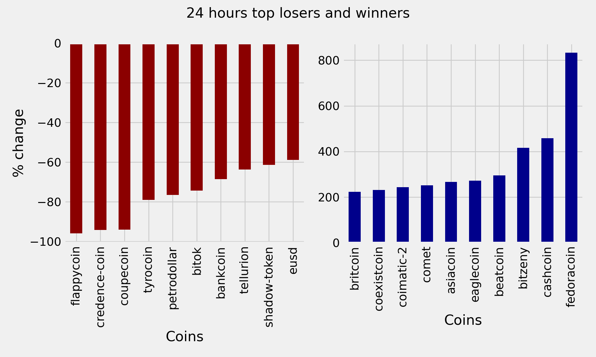

800% daily increase?! That is absolutely insane. Let’s check the weekly changes.

# Sorting percent_change_7d in ascending order
volatility7d = volatility.sort_values("percent_change_7d")

TITLE = "Weekly top losers and winners"

fig, ax = top10_subplot(volatility7d.percent_change_7d, TITLE);
plt.tight_layout()
plt.show()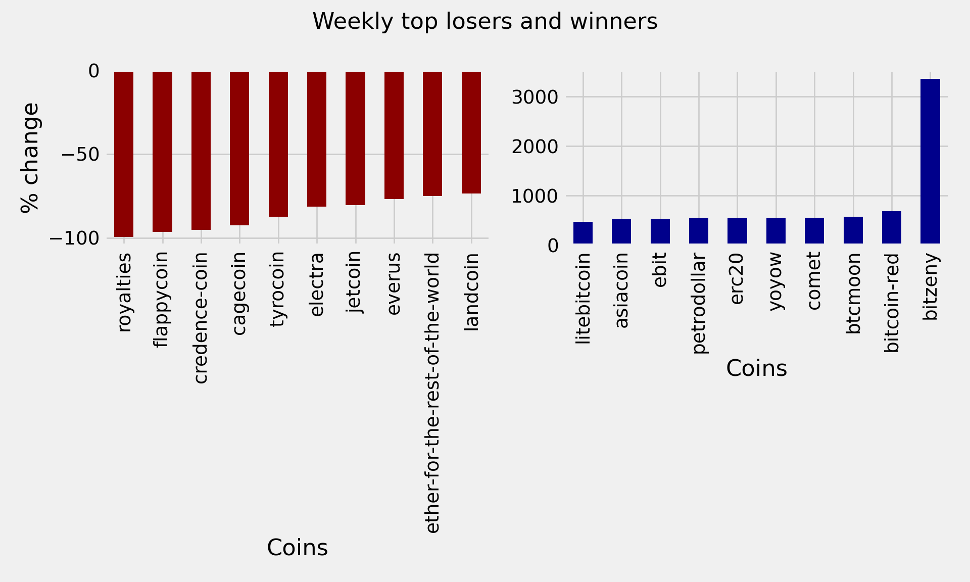

Large Coins

The names of the cryptocurrencies above are quite unknown, and there is a considerable fluctuation between the 1 and 7 days percentage changes. As with stocks, and many other financial products, the smaller the capitalization, the bigger the risk and reward. Smaller cryptocurrencies are less stable projects in general, and therefore even riskier investments than the bigger ones. Cryptocurrencies are a new asset class, so they are not directly comparable to stocks. Furthermore, there are no limits set in stone for what a “small” or “large” stock is. Finally, some investors argue that bitcoin is similar to gold. I just defined the “large” as 10 billion market capitalization. In the next chunk you can see the biggest coins (2017).

# Coins with more than 10 billion market capitalization
largecaps = cap.query("market_cap_usd > 1E+10")


largecaps

##              id  market_cap_usd
## 0       bitcoin    2.130493e+11
## 1      ethereum    4.352945e+10
## 2  bitcoin-cash    2.529585e+10
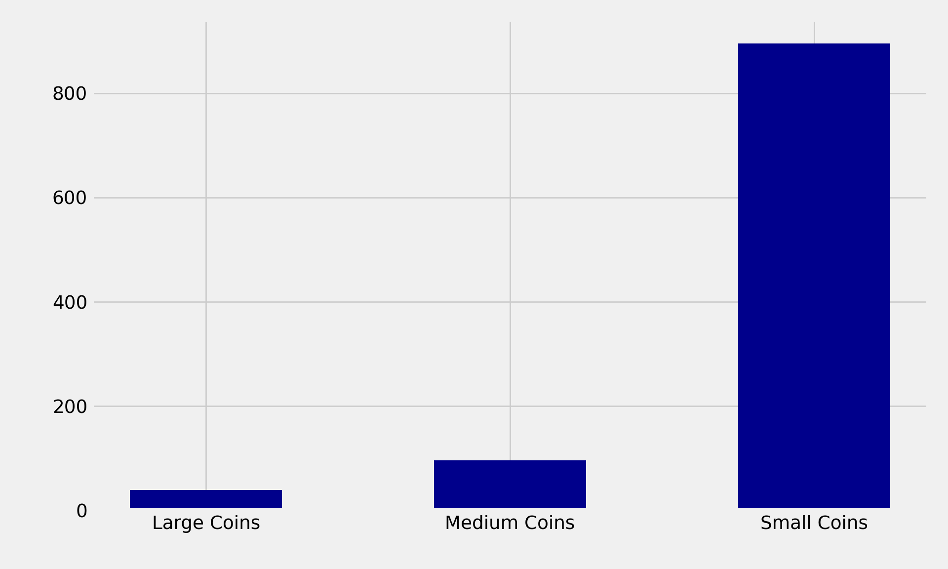
## 3          iota    1.475225e+10

Most coins are tiny. As you can see in the following bar chart most crypto-coins are small. The categories are like the following * Large is more than 300.000.000 in market_cap_usd * Medium is more or equal to 50.000.000 in market_cap_usd * Small is less than 50.000.000 in market_cap_usd

def capcount(query_string):
    return cap.query(query_string).count().id

# Labels for the plot
LABELS = ["Large Coins", "Medium Coins", "Small Coins"]

large = capcount("market_cap_usd > 3E+8")

medium = capcount("market_cap_usd >= 5E+7 & market_cap_usd < 3E+8")

small =  capcount("market_cap_usd < 5E+7")

values = [large, medium, small]

# Plotting
plt.bar(range(len(values)), values, tick_label=LABELS, color="darkblue", width= 0.5);
plt.tight_layout()
plt.show()