Probabilities in Squid Game's Bridge Game- Binomial Distribution
Max Lang / 2021-10-25
Squid Game is still on a huge hype recently. I also watched the show and could not help but notice that in at least one game probability plays a major role.
Spoiler alert
For everybody who hasn’t watched the show yet, the best way to understand this article is to get on Netflix and watch it. Once you’re done watching Squid Game, come back and read this post! ;). Otherwise you can just read this article. Those of you who have finished the series are aware of the glass bridge game, which reduced the number of participants dramatically. The game began with 16 participants and finished with just three. This game features 16 players and an 18-step bridge (two tile options for each step). Each player must go in a certain order. The player must select between two nearly indistinguishable panes of glass at each level. One of the panes is tempered, while the other piece is made of ordinary glass. If you choose wrong you fall to the ground, die and obviously get eliminated.
So let’s get nerdy - how many players would we expect to survive?
So let \(A:\text{Player makes one correct step}\) then the probability \(P(A)= \frac{1}{2}\).
So the probability of one person making 18 correct steps (\(:B\)) (under the assumption that his/her choices are completely random) \(P(B)= (\frac{1}{2})^{18}=\frac{1}{262144}\). This might seem pretty low, but we did not consider the aspect of the game that the second player might have better odds. The second player should know at the very least which tile is safe (or not safe) because of first player’s step. So the second player’s probability for walking safely to the other side of the bridge \(:C\) is \(P(C)= (\frac{1}{2})^{17}= \frac{1}{131072}\). However there is also the possibility that the first player crossing, so we might have to model this game differently.
We now want to find out how many steps each player makes on average until he (sadly) dies.
So let \(X: \text{Player dies (stepping on the wrong tile)}\) and \(Y: \text{Number of steps the player makes until he dies}\) be random variables. Hence the probability is \(P(X)= \frac{1}{2}(=p)\) and we can safely assume that \(Y\) follows a geometric distribution as \(Y\) describes the number of steps until an event (Death) happens. \[ Y \sim G(0.5)\]
plot(dgeom(1:19,0.5), xlab = "Number of steps until player dies (over 18,
passed the bridge)", ylab = "Probability", main= "Distribution of Y ~ G(0.5)")
axis(1, at= seq(from= 1, to= 19, by= 1)) 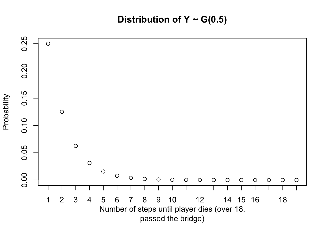
So now if we want to know how many steps one player on average “reveals” until he dies we can just take \(\mu\) of the geometric distribution which is by definition \(\mu = \frac{1}{p}= \frac{1}{0.5} = 2\). So on average one player reveals two steps until he (again sadly) dies. So given that there are 18 pairs of tiles (steps), we would expect \(\frac{\text{Number of steps to pass the bridge}}{\text{Average number of step one player reveals}}= \frac{18}{2}= 9\).
So we would expect about 9 players to die and \(16-9=7\) players to survive and go to the next round of Squid Game.
Well… the Squid Game players did not leave up to our statistical expectations :). Why? One clearly has to remember that the average of the Geometric distribution will move to \(\frac{1}{2}\) for a huge number of “tries”. This can easily be shown if we recall the geometric series which is: \[\sum_{k=0}^\infty r^{k}= \sum_{k=0}^\infty 0.5^{k}=\frac{1}{1-0.5}= 2\]
Normally I would skip the proof and link to Wikipedia, but this proof is actually pretty cool and elegant if one uses the fact that one can rewrite it as a so called telescopic series.
So let’s start with the “proof” using the telescopic series fact. Consider \[f(x)= \frac{r^x}{1-r}\], after a little time of experimenting one finds out that \[f(0)-f(1)=1\], \[r= f(1)-f(2)\] \[r^2= f(2)-f(3)\] and so on. So our series is \[\sum_{k=0}^\infty r^{k} =(f(0)-f(1))+(f(1)-f(2))+(f(2)-f(3))+\dots\] but we know that our \[r=0.5<1\] so therefore \[\lim_{x\to \infty} f(x) =\lim_{x\to \infty} \frac{r^x}{1-r}= 0\] so our series converges to \[f(0)= \frac{1}{1-r}\]. (Not really a proof but the main proof idea.) So of course this is just one “sample” we have in the show, so the mean can be different from the (theoretical) average. Furthermore we said that every player chooses completely randomly where he might go, which is also not really the case in the show. Some players play “dirty” and do not want to give other players the right idea or fall together through one pane. That’s of course not possible in our little theoretical frame here.
Probability of a certain number of players surviving
So now we can ask the question “What’s the probability of \(x\) players surviving?” So in the show \(x= 3\), only three players survived. That means that from our 16 players 13 died. We can now easily calculate how many arrangements are possible for 13 broken squares amongst 18 steps.
choose(18,13) ## [1] 8568So there are 8568 ways to arrange 13 broken squares
amongst 18 steps. We need 13 broken squares which is a probability of
\((\frac{1}{2})^{13}\) and the remaining 5 not to break.
choose(18,13)*(0.5)^13*0.5^5 ## [1] 0.03268433# dbinom(13,18,0.5)\(8568\cdot (\frac{1}{2})^{13} \cdot(\frac{1}{2})^{5}= 3.268 \%\) Another way to go is to calculate the probability that more players would have survived. Let \(Z: \text{Number of tiles broken}\) be a random variables then the probability of them doing better is \(P(Z=12)+ P(Z=11)+ P(Z=10)+ \dots+P(Z=0)\). As some of you might have already guessed from the way of calculating the probability of 3 players surving Z follows a binomial distribution. \[Z\sim B(18,0.5)\]
plot(dbinom(0:18, size= 18,prob = 0.5),type='h', xlim=
c(0,20), xlab= "Number of broken glass panes", ylab= "Probability", main="Distribution of Z")
axis(1, at= 0:19) 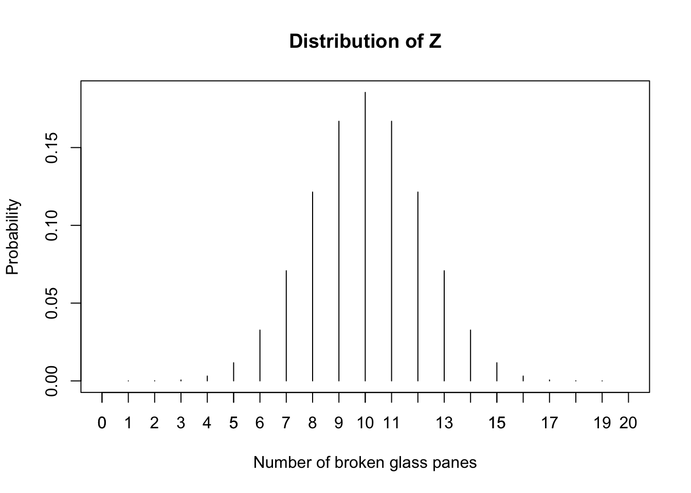
We want the probability that more than 5 tiles were not broken, which is basically \(P(Z\geq5)= 1-P(Z\leq5)= 95.187 \%\)
1-pbinom(5, 18,0.5)## [1] 0.9518738pbinom(5, 18,0.5)## [1] 0.04812622So as you can see the players were unlucky or just pretty stupid to kill each other.
How lucky were our players guessing?
I will not include the “guesses” made by the glassmaker because he clearly was not guessing, he knew what he was doing that is why the Boss switched the lights off.
The players who were guessing made all together 16 guesses of which 5 were correct. (pretty unlucky.) The probability for that is easily calculable
dbinom(5,16,0.5)## [1] 0.066650391-pbinom(5,16,0.5) # Probability of at least 6 right guesses## [1] 0.8949432So a probability of \(6.665\%\) and the probability of at least 6 right guessesis \(89.494 \%\), so the players really were unlucky.
Furthermore one should remember that every time a player was thrown on a glass pane that pane broke. The probability for that is \(0.5^4= 6.25\%\)
So what’s the probability that less than two player survive?
If everybody dies or only one person finishes the game then there would be no need for the last game. The VIPs would probably not like this kind of finish so let’s see how likely this would be. For everybody to die or at least one person to survive we would need at least 15 broken tiles.
1-pbinom(15,18,0.5)## [1] 0.0006561279So the probability for this is really really low, which the organizers probably took into account.
Does the number of players influence the survivors?
During my analysis this question came up in my mind. Because each player will reveal at least on tile for the others (in our theoretical frame), so more players might lead to more surviors.
So let \(n\) be the number of players, \(m\) the number of broken tiles then the formula for the surving player is \[\sum_{m=0}^{n-1}= {18 \choose m}\cdot0.5^m\cdot0.5^{18-m}\cdot (n-m)\]
So let’s check this formula for \(n=16\) players \[\sum_{m=0}^{16-1}= {18 \choose m}\cdot0.5^m\cdot0.5^{18-m}\cdot (16-m)= 7\]
vector <- vector()
for (m in 0:(16-1)){
  vector[m] <- dbinom(m,18,0.5)*(16-m)
}
round(sum(vector))
## [1] 7So pretty close to what we calculated earlier.
Let’s say now we only have half of the 16 players, so 8 players.
vector <- vector()
for (m in 0:(8-1)){
  vector[m] <- dbinom(m,18,0.5)*(8-m)
}
round(sum(vector))
## [1] 0As the absolute numbers are not really helpful we should consider calculating a survival rate for a respective number of players.
survior_calc <- function(nplayers){
  vector <- vector()
for (m in 0:(nplayers-1)){
  vector[m] <- dbinom(m,18,0.5)*(nplayers-m)
}
  return(round(sum(vector)))
}
surviors <- vector
for(i in 1:50){
surviors[i] <- survior_calc(i)
}
squid_frame <- data.frame(list(nplayers= 1:50, surviors= surviors, survival_ratio= surviors/1:50))squid_frame %>%
ggplot(aes(x= nplayers, y= surviors))+
geom_line()+
xlab("Number of players")+
ylab("Survivors")+
ggtitle("Survivors with respect to the number of players")+
theme_minimal()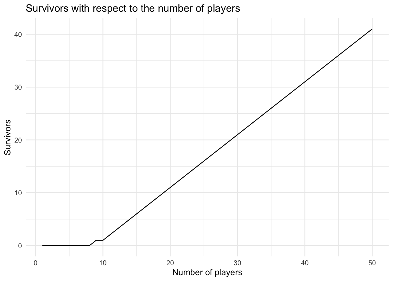
squid_frame %>%
  ggplot(aes(x= nplayers, y= survival_ratio)) +
  geom_line()+
  xlab("Number of players")+
  ylab("Survival %")+
  ggtitle("Survival ratio with respect to the number of players")+
  theme_minimal()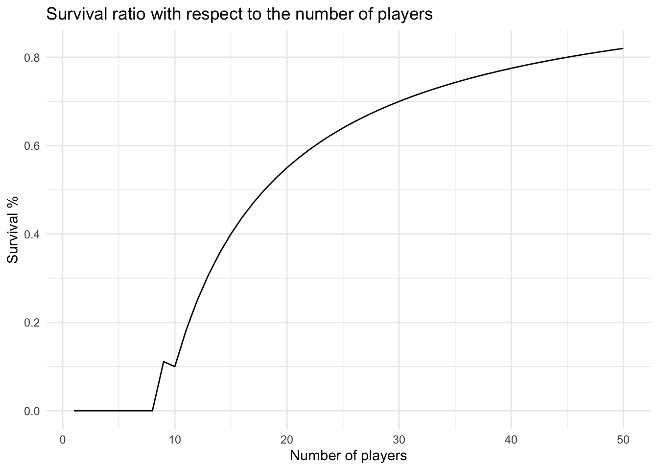
Was this just a waste of time?
Of course not! It was a great way to play with the binomial distribution and actually a lot of fun to think about this bridge game from a statistical standpoint! Furthermore there a lot of problems in the real world that can be modled with a binomial distribution. If you are interested you can check out this video.