Generating random variables
Max Lang / 2021-12-19
Table of contents
- Outline
- The uniform distribution
- Laying the mathematical foundation
- Graphical intuition
- Generating Random Variables / applying the theory
- Final thoughts
Outline
The goal of this post is to illustrate the mathematical beauty of generating random varibales from a simple uniform distribution. (\(U ∼ U [0, 1]\))
We will find out that it is possible to generate complicated random variables and stochastical models from this relatively boring uniform distribution by applying the golden standard: the inverse transform method.
The uniform distribution
First, we will assume that we can generate a sequence of
independent random variables that are uniformly
distributed on the standard interval \([0,1]\)
In R this can simply be done with the command u = runif(100) which returns 100 realizations of
a uniform random variable on (0, 1).
The density will look like this:
However, super strictly speaking, we only have access to pseudo-random (deterministic) numbers, because that’s just how computers work. Of course we have access to modern random number generators (constructed on number theory) and standard tests for uniformity, independence, etc. do not show significant deviations. So I do not want to put too much focus on that aspect (even though it is really interesting.)
So let’s get started with our inversion method.
Laying the mathematical foundation
When do we call a function a cumulative distribution function (cdf)?
From several statistics and probability theory courses you might know that any Function is a cumulative distribution function (cdf) if: - \(F : \mathbb R → [0, 1]\)
\(F\) is increasing monotonously
\(F\) is right continuous
\(F: \mathbb{R} \rightarrow[0,1] \text { with }\lim _{x \rightarrow-\infty} F(x)=0 \text { and } \lim _{x \rightarrow \infty} F(x)=1\)
Inverse transform method and proof of correctness
Let \(F\) be a continuous and strictly increasing \(c d f\) on \(\mathbb{R}\), we can define its inverse \(F^{-1}:[0,1] \rightarrow \mathbb{R}\). Let \(U \sim \mathcal{U}[0,1]\) then \(X=F^{-1}(U)\) has cdf \(F\). Quick Proof / Verification: \[ \begin{aligned} \mathbb{P}(X \leq x) &=\mathbb{P}\left(F^{-1}(U) \leq x\right) \\ &=\mathbb{P}(U \leq F(x)) \\ &=F(x) \end{aligned} \]
So now let \(F\) be a cdf on \(\mathbb{R}\) and define its generalized inverse \(F^{-1}:[0,1] \rightarrow \mathbb{R}\) \[ F^{-1}(u)=\inf \{x \in \mathbb{R} ; F(x) \geq u\} \] Let \(U \sim \mathcal{U}[0,1]\) then \(X=F^{-1}(U)\) has cdf \(F\).
Graphical intuition
OK, that was a little math for the start, but what did we actually figure out above? We basically take advantage of the fact, that any \(cdf\) functions only returns \(y\)-values between \([0,1]\). (You can go back and check under “When do we call a function a cumulative distribution function (cdf)?” to check.) This intervall from \([0,1]\) is also exactly the domain of our uniform distribution. (Check the plot).
So what happens graphically if we take the inverse?
Let’s take a look at this exponential density plot as well as on the plot of cdf.
So what we do is to assign every value on the y axis a value on the x axis, obviously this is just how an inverse function works. The important point however is, that our returned \(x\) values now follow the same distribution as the cdf did, so in this case a exponential distribution.
Generating Random Variables / applying the theory
Example: Weibull Distribution
So now that we understood the math laid out before we can apply it. Let’s try to find the inverse of a weibull distribution function which is basically a more general case of the exponential function as for \(\alpha=1\) it is the exponential distribution. Weibull distribution. Let \(\alpha, \lambda>0\) then the Weibull cdf is given by \[ u= F(x)=1-\exp \left(-\lambda x^{\alpha}\right), x \geq 0 \]
Now let’s start solving for \(u\): \[ \begin{aligned} u &=F(x) \Leftrightarrow \log (1-u)=-\lambda x^{\alpha} \\ & \Leftrightarrow x=\left(-\frac{\log (1-u)}{\lambda}\right)^{1 / \alpha} \end{aligned} \] Because of \((1-U) \sim \mathcal{U}[0,1]\) when \(U \sim \mathcal{U}[0,1]\) we can now use this to define our random variable that follows a weibull distribution. \[ X=\left(-\frac{\log U}{\lambda}\right)^{1 / \alpha} . \]
This formula basically is the mathematical way of describing what we did before. It assigns every value on the y-Axis a value on the x-Axis. Hence, it returns our wanted random variable which follows a weibull distribution. Cool!
So we can check if this is actually true (of course it is because it’s mathematically correct lol).
Implementation in R / verification
weibull_simulation <- function(n, alpha= 1, rate= 0.5){
  ((-log((1-runif(n)))/rate))^(1/alpha)
}

plot(weibull_simulation(100, alpha = 1, rate= 3), main= "Weibull Simulation", ylab= "Values")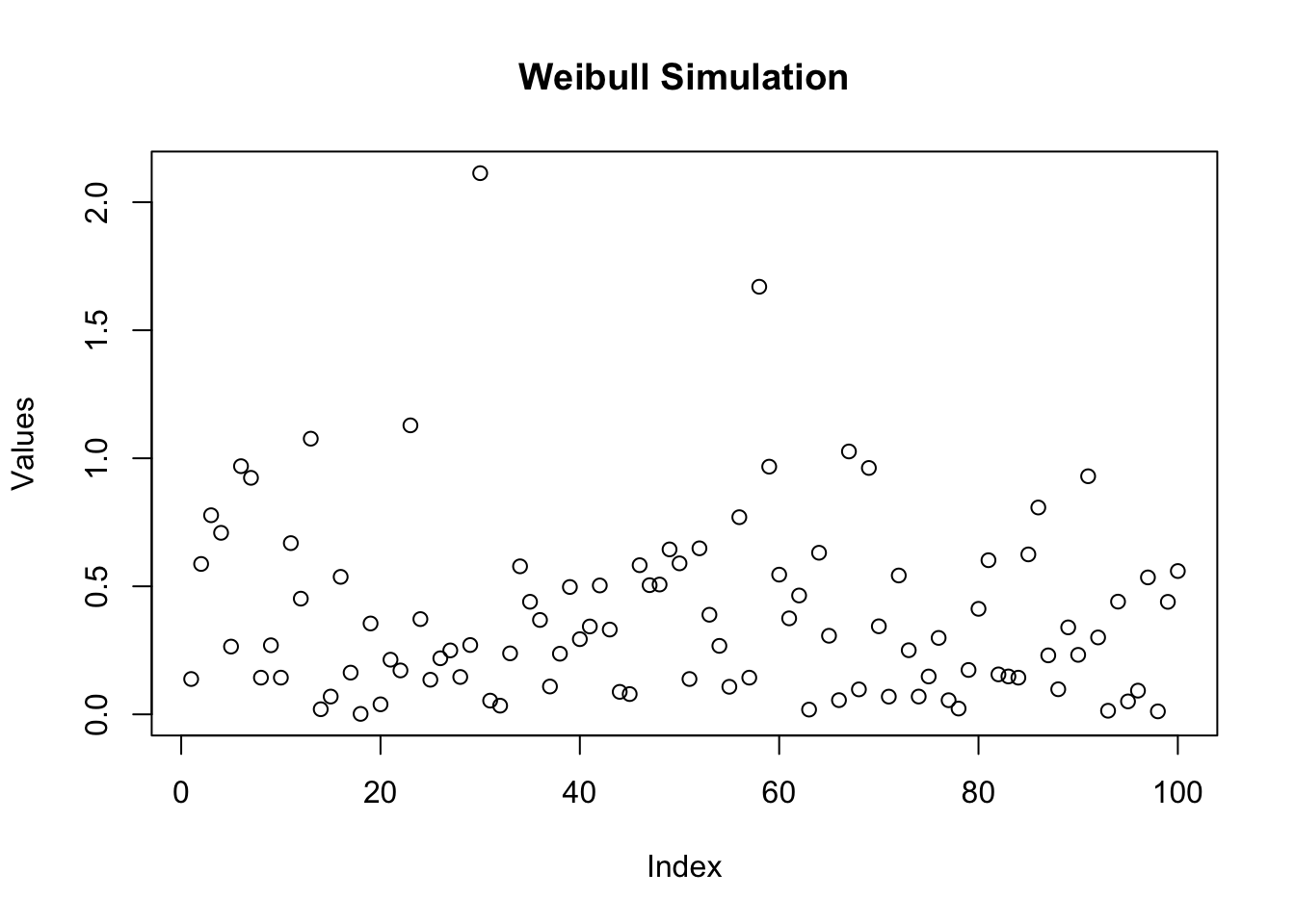
hist(weibull_simulation(20000, alpha = 1, rate = 3), probability = TRUE, n=100, main= "Histogram of the distribution", ylab= "Density", xlab = "Values")
lines(seq(0,5,length=20000),dexp(seq(0,5,length=20000),rate = 3), col= "red")
legend("topright",legend= "Density of \nexponential distribution",col = "red", fill= "red", cex= 0.6)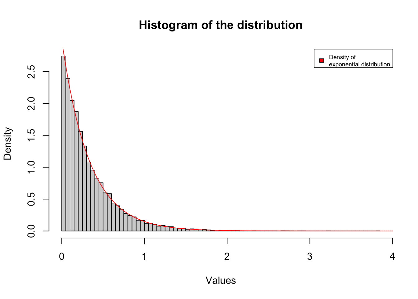 And indeed for a large
 nit follows an exponential distribution like it should.
Of course this also works for other parameters:
hist(weibull_simulation(200000, alpha = 2, rate = 1), probability = TRUE, n=100, main= "Histogram of the distribution", ylab= "Density", xlab = "Values")
lines(seq(0,5,length=20000),dweibull(seq(0,5,length=20000), shape = 2, scale = 1), col= "red")
legend("topright",legend= "Density of \nweibull distribution",col = "red", fill= "red", cex= 0.6)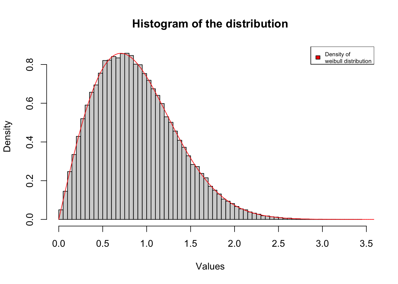
Final thoughts
This is pretty awesome and fascinating in my opinion. This also works for other distributions like the geometric distribution or the cauchy distribution for example. The only point this method can not be used is if we do not know the cdf of the distribution like for example with the normal distribution. In this case we would need to take a look at a more generalized idea like transformation methods, e.g. the Box-Muller Algorithm. On the other hand, it is possible to approximate the quantile function of the normal distribution extremely accurately using moderate-degree polynomials, and in fact the method of doing this is fast enough that inversion sampling is now the default method for sampling from a normal distribution in the statistical package R.