Random Forests
Max / 2023-01-18
Variable Importance from mlr3
Data prep
data("Servo")
servo <- Servo %>%
  mutate_at(c("Pgain", "Vgain"), as.character) %>%
  mutate_at(c("Pgain", "Vgain"), as.numeric)
head(servo)
## Motor Screw Pgain Vgain Class
## 1 E E 5 4 4
## 2 B D 6 5 11
## 3 D D 4 3 6
## 4 B A 3 2 48
## 5 D B 6 5 6
## 6 E C 4 3 20train_size <- 2/3
set.seed(1333)
train_index <- sample(
x = seq(1, nrow(servo), by = 1),
size = ceiling(train_size * nrow(servo)), replace = FALSE
)
train_1 <- servo[ train_index, ]
test_1 <- servo[ -train_index, ]task <- TaskRegr$new(id = "servo", backend = train_1, target = "Class")
lrn1 <- lrn("regr.ranger", importance = "impurity")
lrn1$train(task = task)
filter <- mlr3filters::flt("importance", learner = lrn1)
filter$calculate(task)
var <- as.data.table(filter)
ggplot(data = var, aes(x = feature, y = score)) + geom_bar(stat = "identity") +
ggtitle(label = "Variable Importance with mlr3") +
labs(x = "Feature", y = "Variable Importance")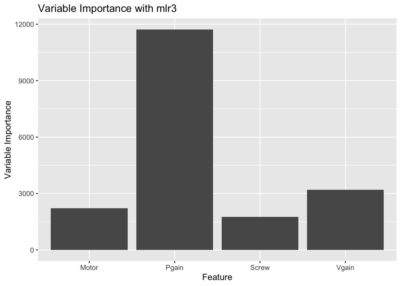
Decision Regions CART vs. Random Forest
Data used:
spiral <- mlbench::mlbench.spirals(1000, cycles = 2, sd = 0.5)
p <- ggplot(data = as.data.frame(spiral$x), aes(
  x = V1, y = V2,
  colour = spiral$classes
)) +
  geom_point()
p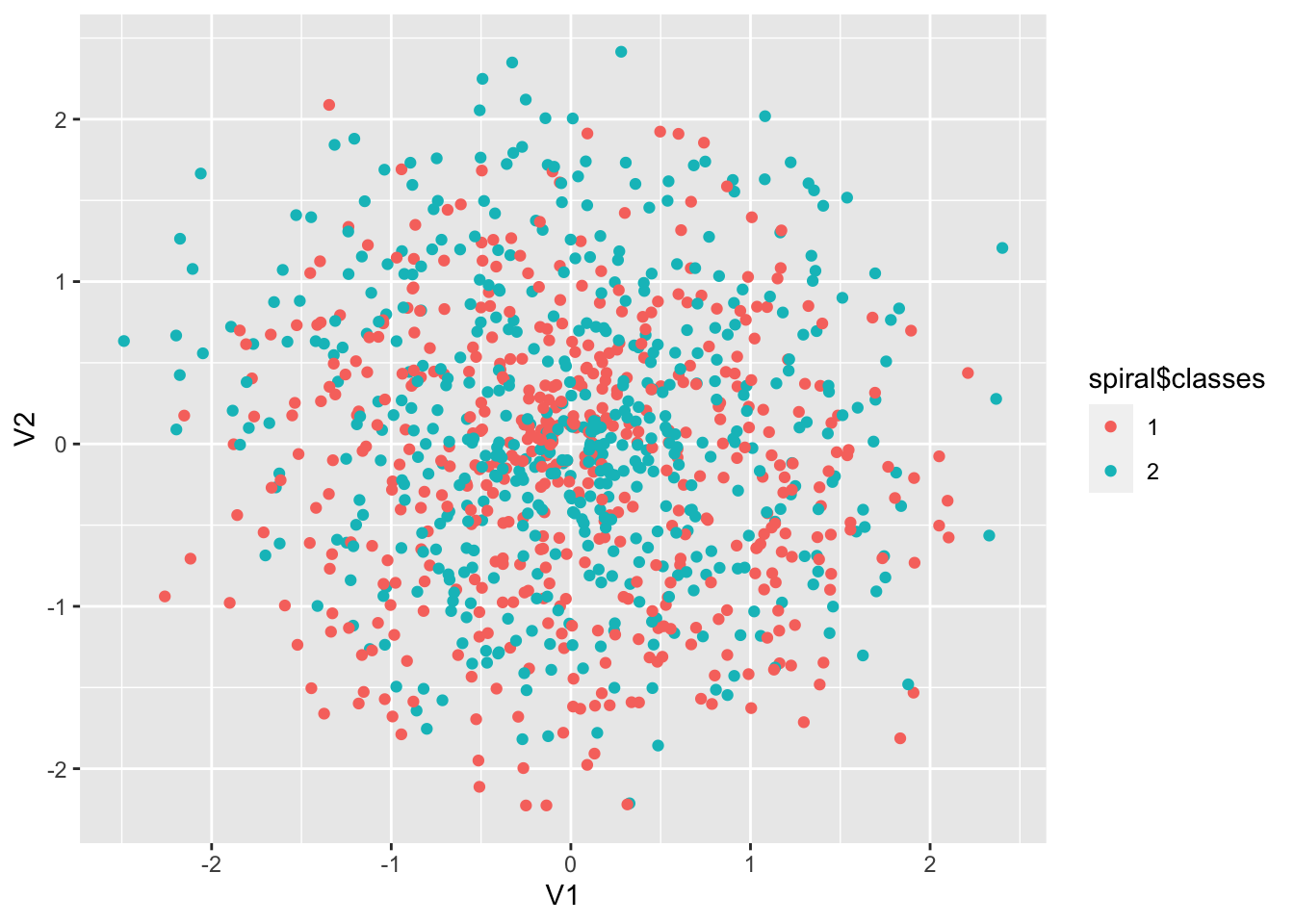
Decision regions CART
spiral_data <- data.frame(spiral$x, y = factor(spiral$classes))
colnames(spiral_data) <- c("x1", "x2", "y")

features <- c("x1", "x2")
spiral_task <- TaskClassif$new(
  id = "spirals", backend = spiral_data,
  target = "y"
)
plot_learner_prediction(
  lrn("classif.rpart", predict_type = "prob"),
  spiral_task
)
## INFO [17:14:32.188] [mlr3] Applying learner 'classif.rpart' on task 'spirals' (iter 1/1)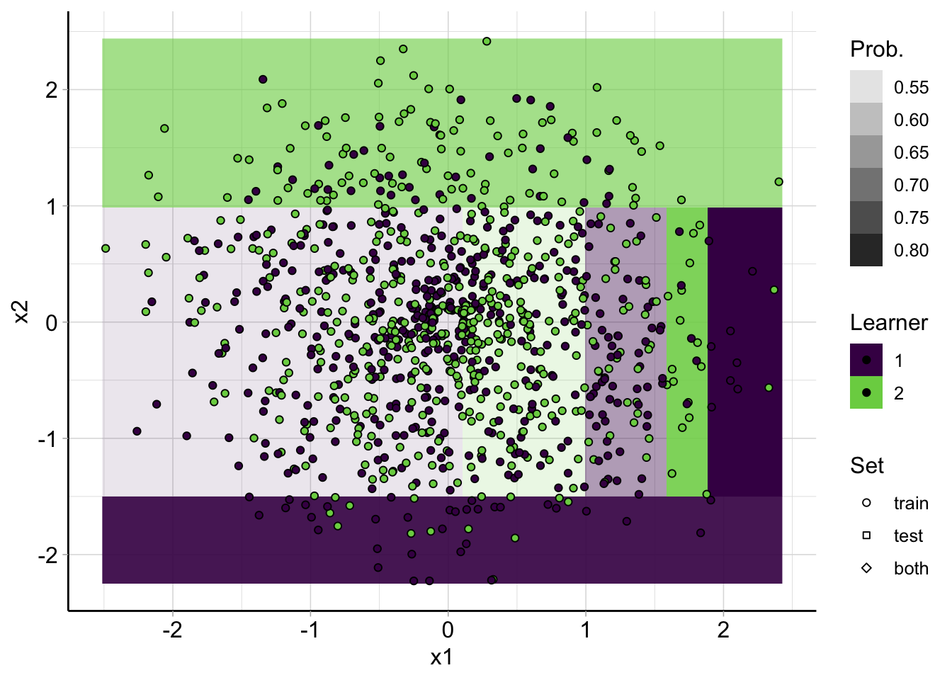
Decision regions Random Forest
plot_learner_prediction(
  lrn("classif.ranger", predict_type = "prob"),
  spiral_task
)
## INFO [17:14:33.402] [mlr3] Applying learner 'classif.ranger' on task 'spirals' (iter 1/1)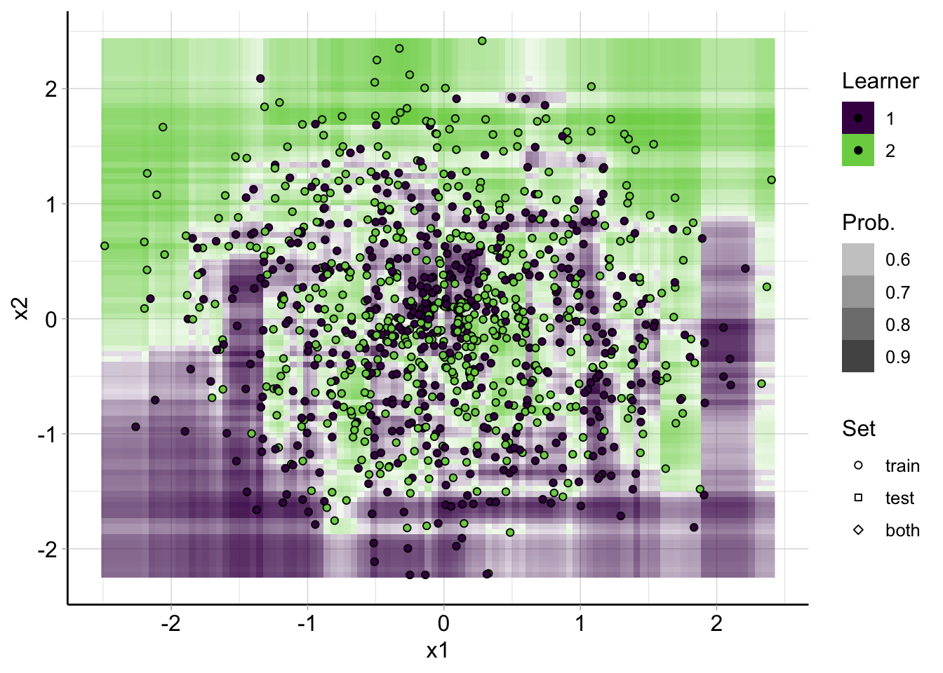
Proximity measures in Random Forests
set.seed(1337)
spiral_rf <- randomForest(
  x = spiral$x, y = spiral$classes,
  ntree = 1000,
  proximity = TRUE, oob.prox = TRUE,
)
spiral_proximity <- spiral_rf$proximity
spiral_proximity[1:5, 1:5]
## [,1] [,2] [,3] [,4] [,5]
## [1,] 1.0000000 0.0078125 0 0 0
## [2,] 0.0078125 1.0000000 0 0 0
## [3,] 0.0000000 0.0000000 1 0 0
## [4,] 0.0000000 0.0000000 0 1 0
## [5,] 0.0000000 0.0000000 0 0 1Proximity MDS (Multidimensional Scaling)
proximity_to_dist <- function(proximity) {
  1 - proximity
}
spiral_dist <- proximity_to_dist(spiral_proximity)
spiral_dist[1:5, 1:5]
## [,1] [,2] [,3] [,4] [,5]
## [1,] 0.0000000 0.9921875 1 1 1
## [2,] 0.9921875 0.0000000 1 1 1
## [3,] 1.0000000 1.0000000 0 1 1
## [4,] 1.0000000 1.0000000 1 0 1
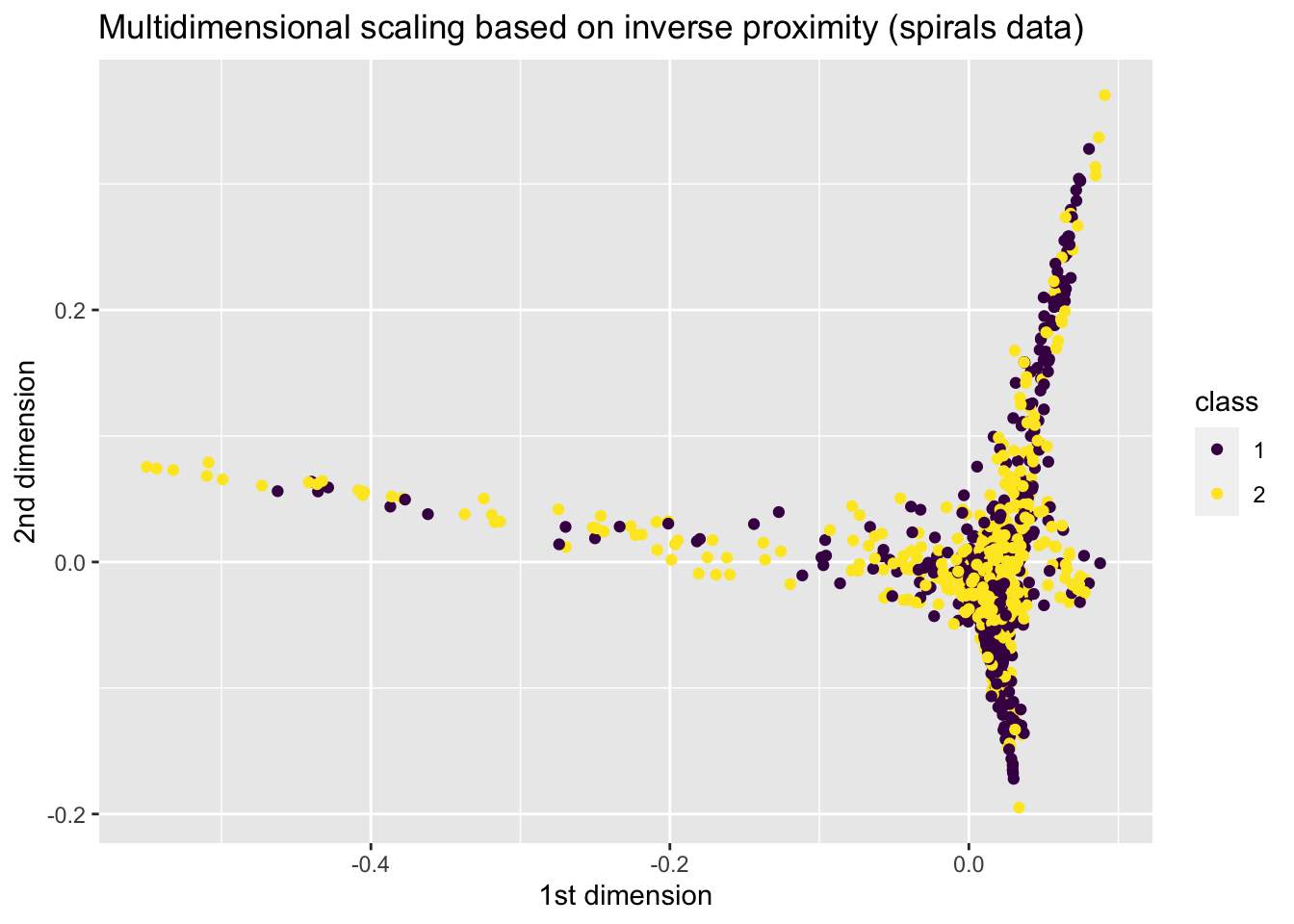
## [5,] 1.0000000 1.0000000 1 1 0spiral_mds <- as.data.frame(cmdscale(spiral_dist))
spiral_mds$class <- spiral$classes
# plot the result, sweet
plot <- ggplot(data = spiral_mds, aes(x = V1, y = V2, colour = class)) +
geom_point() +
labs(
x = "1st dimension", y = "2nd dimension",
title = "Multidimensional scaling based on inverse proximity (spirals data)"
)+
scale_colour_viridis_d()
plot