ABC is particularly useful when dealing with complex models where the likelihood function is difficult or impossible to calculate. To understand its significance, let’s delve into a worked example where normal methods do not suffice, and the application of ABC becomes invaluable.

Consider a scenario in data analysis where we need to estimate parameters of a statistical model, but the likelihood function, which is central to Bayesian inference, is either too complex or unknown. Traditional methods like Maximum Likelihood Estimation (MLE) or standard Bayesian approaches hinge on the ability to calculate this likelihood, which might be unfeasible in many real-world situations.

For example \(5 \sim 6\) in Table \(\ref{tab:ising-1}\) and the neighbors of cell 9 are \(\{8,6\}\). Let \[ \# y=\frac{1}{2} \sum_{i=1}^{m^2} \sum_{j \sim i} \mathbb{I}_{Y_j \neq Y_i} \] where \(\sum_{j \sim i}\) sums over all \(j\) such that \(j\) is a neighbor of \(i\). Here #y counts the number of “disagreeing neighbors” in the binary image \(Y=y\). In the example in Table \(\ref{tab:ising-1}\) we have #y=4.

\[ p(y \mid \theta)=\exp (-\theta \# y) / c(\theta) . \]

It has a free boundary because cells on the edge have no neighbors beyond the edge. Here \(\theta \geq 0\) is a positive smoothing parameter and \[ c(\theta)=\sum_{y \in \mathcal{Y}} \exp (-\theta \# y) \] is . There are \(2^{m^2}\) terms in the sum, and no one can solve it (it is an important model in physics, so many have looked at this).

Suppose we have image data \(Y=y_{o b s}\) with \(y_{o b s} \in\{0,1\}^{m^2}\) and we want to estimate \(\theta\). Consider doing MCMC targeting \(\pi\left(\theta \mid y_{o b s}\right)\) with some prior \(\pi(\theta)\). Choose a simple proposal for the scalar parameter \(\theta\), say \(\theta^{\prime} \sim U(\theta-a, \theta+a), a>0\). The acceptance probability is \[ \begin{aligned} \alpha\left(\theta^{\prime} \mid \theta\right) & =\min \left\{1, \frac{p\left(y \mid \theta^{\prime}\right) \pi\left(\theta^{\prime}\right)}{p(y \mid \theta) \pi(\theta)}\right\} \\ & =\min \left\{1, \frac{c(\theta)}{c\left(\theta^{\prime}\right)} \times \exp \left(\left(\theta-\theta^{\prime}\right) \# y\right) \times \frac{\pi\left(\theta^{\prime}\right)}{\pi(\theta)}\right\} \end{aligned} \] and although \(p(y)\) cancels, This leads us to the following definition.

Doubly intractable distributions present a significant challenge in statistical computing, primarily encountered in Bayesian analysis. These distributions are characterized by a likelihood function that includes an intractable normalizing constant, which itself depends on the parameters of interest. This dependency creates a ‘double’ intractability: not only is the likelihood intractable, but so is its normalization. (doubly intractable problems) If for \(y_{o b s} \in \mathcal{Y}\) and \(\theta, \theta^{\prime} \in \Omega\) either of the ratios \(p\left(y_{o b s} \mid \theta\right) / p\left(y_{o b s} \mid \theta^{\prime}\right)\) or \(\pi(\theta) / \pi\left(\theta^{\prime}\right)\) cannot be evaluated then the posterior is said to be doubly intractable.

ABC provides a pathway to handle these doubly intractable problems. By comparing simulated and observed data without the need to directly calculate the likelihood or its normalizing constant.

In ABC, the goal is to approximate the posterior distribution of the parameters, which in traditional Bayesian analysis would be derived using Bayes’ theorem and the likelihood function. ABC does this indirectly. It and . . This process results in an approximation of the posterior distribution, which is why it’s often referred to as approximating the approximated posterior.

The ABC methodology can be broken down into a stepwise process:

We would not make an approximation unless it helped us somehow, here we approximate our target \(p\left(\theta \mid y_{o b s}\right)\). The point is that, if \(\delta\) is not too small, \(\pi\left(\theta \mid Y \in \Delta_\delta\left(y_{o b s}\right)\right)\) is often very easy to sample, and we can do it “perfectly” using rejection, even in cases where the observation model is very complex. Rejection-samples are iid and distributed according to the target, so there are no issues with burn-in or mixing as in MCMC.

1. \(\operatorname{Set} n=0\)
2. Set \(n \leftarrow n+1\). Simulate \(\theta_n \sim \pi(\cdot)\) and \(y_n \sim p\left(\cdot \mid \theta_n\right)\)
3. If \(y_n \in \Delta_\delta\left(y_{o b s}\right)\) stop and return \(\Theta_{A B C}=\theta_n, Y_{A B C}=y_n\) and \(N=n\) else go to step 2.

The ABC-Rejection Algorithm returns samples \(\left(\Theta_{A B C}, Y_{A B C}, N\right)\) with \(\Theta_{A B C} \sim \pi\left(\cdot \mid Y \in \Delta_\delta\left(y_{o b s}\right)\right)\).

Run this algorithm \(T\) times returning \(\lambda^{(1)}, \lambda^{(2)}, \ldots, \lambda^{(T)}\). These are samples from \(\pi_{A B C}\left(\lambda \mid y_{o b s}\right)\).

When Approximate Bayesian Computation (ABC) is applied, it often yields samples that approximate the posterior distribution of interest. However, due to the approximate nature of ABC, these samples may not be as close to the true posterior as desired, particularly when the tolerance level δ is not small enough. Regression adjustment is a post-processing step that aims to improve the approximation by aligning the sampled parameters more closely with the true posterior distribution.

The intuitive idea behind regression adjustment is to “correct” the sampled parameters by accounting for the discrepancy between the simulated summary statistics and the observed summary statistics. Essentially, it involves fitting a regression model where the sampled parameters are the response variable, and the discrepancy is the predictor. The fitted regression model is then used to adjust the ABC samples towards the region where the simulated data is more similar to the observed data.

Consider the pairs \((\theta, y) \sim \pi(\theta) p(y \mid \theta)\) generated by ABC. Conditional on \(y\) we have \(\theta \sim \pi(\theta \mid y)\). We will adjust this distribution by making a transformation \(\theta^{(a d j)}=f(\theta)\) so that \(\theta^{(a d j)} \sim \pi\left(\cdot \mid y_{o b s}\right)\). This is not achievable in general. We will set out some assumptions under which this operation is exact and straightforward, and use this to motivate the method when the assumptions do not hold but are satisfied to a good approximation. We consider scalar \(\theta \in \mathbb{R}\) to simplify notation (in regression with a multivariate response, \(\beta\) below is a matrix). The idea extends easily to \(\theta \in \mathcal{R}^p\).

Let \(\theta \sim \pi(\cdot \mid y)\) and \(\theta^{\prime} \sim \pi\left(\cdot \mid y_{o b s}\right)\). Let \(s=S(y)\) and \(s_{o b s}=S\left(y_{o b s}\right)\).

One of the main reasons for doing regression adjustment is that it allows us to take \(\delta\) quite large and fix the poor approximation using the regression adjustment. Some experimentation is usually necessary (to choose \(\delta\) small enough so the approximation doesnt change significantly when we make it smaller). We like to take \(\delta\) large as more samples are retained (in Proposition 3.15 in the ABC-rejection algorithm we throw out samples if \(D\left(S(y), S\left(y_{o b s}\right)\right)>\delta\) ), or alternatively, shorter runtimes at a fixed sample size.

# Load necessary libraries
library(coda)
library(lattice)
set.seed(42)
# Estimating Poisson Mean using ABC

# Set true lambda and sample size
trueLambda <- 2
sampleSize <- 5

# Example data
dataY <- c(1, 1, 2, 2, 3)
priorAlpha <- 1
priorBeta <- 1

numSimulations <- 100000
acceptedLambdas <- numeric(0)
tolerance <- 1  # Define a tolerance level for accepting lambda

for (i in 1:numSimulations) {
  sampledLambda <- rgamma(1, shape = priorAlpha, rate = priorBeta)
  simulatedData <- sort(rpois(sampleSize, lambda = sampledLambda))
  if (sum((simulatedData - dataY)^2) <= tolerance) {  # Less strict condition
    acceptedLambdas <- c(acceptedLambdas, sampledLambda)
  }
}

# Plotting the results
histogramObject <- hist(acceptedLambdas, 20, plot = FALSE)
plot(histogramObject$mids, histogramObject$density, ylim = c(0, 1.1), type = 'l', col = 2, xlab = 'Lambda', ylab = 'Posterior', lwd = 2)
lines(histogramObject$mids, dgamma(histogramObject$mids, shape = priorAlpha + sum(dataY), rate = priorBeta + sampleSize), lwd = 2)

# ABC with mean as statistic
numABC <- 10000
lambdaABC <- meanABC <- numeric(0)
meanDataY <- mean(dataY)
toleranceDelta <- 0.5
for (i in 1:numABC) {
  sampledLambda <- rgamma(1, shape = priorAlpha, rate = priorBeta)
  simulatedData <- sort(rpois(sampleSize, lambda = sampledLambda))
  if (abs(mean(simulatedData) - meanDataY) < toleranceDelta) {
    lambdaABC <- c(lambdaABC, sampledLambda)
    meanABC <- c(meanABC, mean(simulatedData))
  }
}
histogramABC <- hist(lambdaABC, 50, plot = FALSE)
lines(histogramABC$mids, histogramABC$density, type = 'l', col = 3, lwd = 2)

# Regression correction for ABC
adjustLambda <- function(lambda, simMeans, dataMean) {
  regressionCoef <- coef(lm(lambda ~ simMeans))[2]
  adjustedLambda <- lambda + regressionCoef * (dataMean - simMeans)
  return(adjustedLambda)
}

lambdaAdjusted <- adjustLambda(lambdaABC, meanABC, meanDataY)
histogramAdjusted <- hist(lambdaAdjusted, 50, plot = FALSE)
lines(histogramAdjusted$mids, histogramAdjusted$density, type = 'l', col = 3, lwd = 2, lty = 2)
legend("topright", 
       legend = c("Rejection Sampling", "True Posterior", "ABC Result", "ABC Adjusted"),
       col = c(2, 1, 3, 3),
       lwd = 2,
       lty = c(1, 1, 1, 2))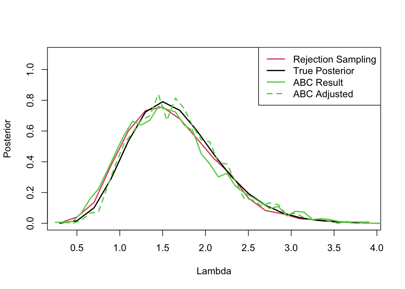

import numpy as np
import matplotlib.pyplot as plt

# Parameters for the Gaussian distributions
std_dev = np.sqrt(2)  # Standard deviation set to sqrt(2) to get variance 2
y_selected_values = [2, 4, 6]  # Selected y values
modes = [0, 2, 4]  # Modes for the Gaussian distributions at each y value (identical to the means for a Gaussian)

# Create a figure and axis
fig, ax = plt.subplots(figsize=(10, 6))

# Plot each Gaussian distribution vertically for the selected y values
for y, mode in zip(y_selected_values, modes):
    x = np.linspace(mode - 4 * std_dev, mode + 4 * std_dev, 300)
    y_gaussian = np.exp(-(x - mode)**2 / (2 * std_dev**2)) / (std_dev * np.sqrt(2 * np.pi))
    ax.plot(y_gaussian + y, x, color='blue')  # Shift the Gaussian to the y position

    # Add a point for the mean of the distribution
    ax.plot(y, mode, 'ro')  # 'ro' is the matplotlib code for a red circle

# Plot a linear dashed line through the red dots (means of the distributions)
ax.plot(y_selected_values, modes, 'k--')

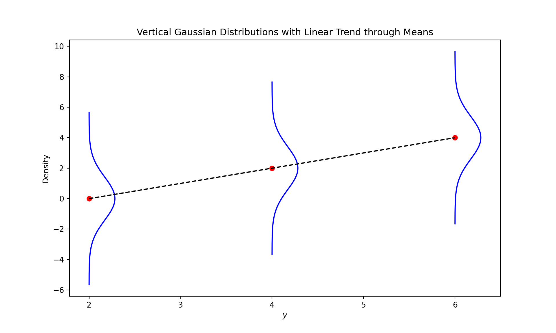
# Set titles and labels
ax.set_title('Vertical Gaussian Distributions with Linear Trend through Means')
ax.set_xlabel('$y$')
ax.set_ylabel('Density')

# Show the plot
plt.show()