HTH vs. HTT - The attempt of an explanation

Max Lang / 2021-04-25

Question

This question was asked during the really interesting TedTalk about statistics by Peter Donelly.

Consider two Patterns HTH vs HTT. Which of the following is true?

a) The average number of tosses until HTH is larger than the average number of tosses until HTT

b) The average number of tosses until HTH is the same as the average number of tosses until HTT

c) The average number of tosses until HTH is smaller than the average number of tosses until HTT

First one might think b) is the correct answer. After a second thought one notices that the sequence HTH overlaps itself. Let’s say one got HTHTH it is clear that one got two occurrences of HTH in only five coin tosses. (HTHTH and HTHTH).

Taking a look at the second sequence HTT one will find out that there is not such an overlap. Therefore one might think that HTH is more likely than HTT which is not the case as shown in the code chunk below.

One should note that we are either looking for HTT or (exclusive) for HTH.
We only flip until the pattern which we are looking for got hit.

set.seed(10)

fair_coin <- c('H','T')

seek <- function(seq) {
  # Flipping the coin three times
    result <- sample(x= fair_coin, size= 3,replace=TRUE)
  # Defining the minimum Number of flips (three)
    flips <- 3
  # Setting  issed to true so while loop iterates at least one time
    missed <- TRUE
  
    while (missed == TRUE) {
      # If all our elements in the vector are the same as the sequence we seek stop the loop
        if (all(seq == result)) {
            missed <- FALSE
        }
      # Recycle last two elements and flip again once (important)
        else {
            result <- c(result[2],result[3], sample(x= fair_coin, size= 1, replace= TRUE))
            flips <- flips + 1
        }
    }
    return(flips)
}
# Setting the number of flips of t experi
n <- 10000

experiment <- data.frame("HTH"=rep(NA,n),"HTT"=rep(NA,n))

HTH <- c('H','T','H')
HTT <- c('H','T','T')

for (i in 1:n) {
    experiment[i,] <- c(seek(HTH),seek(HTT))    
}
# Average number of flips
summary(experiment)

##       HTH             HTT        
##  Min.   : 3.00   Min.   : 3.000  
##  1st Qu.: 4.00   1st Qu.: 5.000  
##  Median : 8.00   Median : 7.000  
##  Mean   :10.04   Mean   : 8.054  
##  3rd Qu.:13.00   3rd Qu.:10.000  
##  Max.   :87.00   Max.   :47.000

The attempt of an explanation:

Let’s suppose the following scenarios.

Looking for the sequence HTH

HTH

The simplest scenario in which we win right away.

HTT

Because of the last T in the sequence one needs to start tossing until one gets another H to “start” the HTT sequence.

Comment 1:

Let’s suppose one already got HT. If the next toss is H one found the sequence and is done. If it’s a T, one has to start all over again: since the last two tosses were TT one now needs the full HTH.

Looking for HTT

HTT

Again the simplest scenario in which we win right away.

HTH

Because we are looking for HTT we did not win in this case. However, and this is the important, at this stage one does not need to toss the coin again in order to find the starting token H.

Comment 2:

Let’s suppose again one already got HT. If the next toss is T, one found the sequence. If it is a H, this is just a minor setback, because one now got HTH (while seeking the HTT sequence); however, now one already has the H and just needs two T in a row ( TT ). Moreover if the next toss is an H this is not such a big setback again, because H is the start of the sequence we are looking for, just like before. A T would make our “situation” even better and so on…

Therefore answer a) The average number of tosses until HTH is larger than the average number of tosses until HTT.

Experiment 2

After we put in some thought, we wanted to find how the probabilities of those two sequences behave if we adjust the experiment.

Now we will throw a coin 100 Times and note down each outcome. The result of each run of the experiment will therefore be a line/string looking e.g like this one “HTHTTTHHHTHTHTHTHT…”, containing in total 100 characters. After this we go through our 100 character long string and check for the following patterns.

HTH
HTT

Note that HTH can overlap itself. For example HTHTH is counted as HTHTH and HTHTH - two sequences for HTH. HTT does not have this characteristic.

The Question is which of the following statements is true:

The number of times HTH is in our string is more than the number of times HTT occurs
The number of times HTH is in our string is less than the number of times HTT occurs
The number of times HTH is in our string is equal to the number of times HTT occurs

Let’s make a simple simulaton in R to find out the correct answer. We first defined this function to simulate or experiment.

library(ggplot2)

count.pattern <- function(pattern,
                          n_flips = 100,
                          coins = rbinom(n_flips, 1, 0.5)) {
  hits = 0
  for (i in 1:(n_flips - 2)) {
    # TRUES are counted as 1 in R, this allows the following step
    if (sum(coins[i:(i + 2)] == pattern) == 3) {
      hits = 1 + hits
    }
  }
  hits
}

Run the experiment

# Encoded 0 = H and 1 = T
HTH = c(0, 1, 0)
HTT = c(0, 1, 1)
TTT = c(1, 1, 1)

n_flips =  100

# Running the experiment 10000 times seeking HTH, HTT and TTT
results = data.frame(
  HTH = replicate(10000, count.pattern(HTH, n_flips)),
  HTT = replicate(10000, count.pattern(HTT, n_flips)),
  TTT = replicate(10000, count.pattern(TTT, n_flips))
)
summary(results)[4,]

##               HTH               HTT               TTT 
## "Mean   :12.27  " "Mean   :12.25  "  "Mean   :12.2  "

The means at 10000 trials are close enough that we can safely assume that the average amount of successes is the same, no matter which pattern.

However, their distribution is not:

Plotting the histograms of all three patterns

ggplot(tidyr::pivot_longer(results,
                           c("HTH", "HTT", "TTT"),
                           names_to = "pattern",
                           values_to = "value"),
       aes(value)) +
  geom_histogram(binwidth = 0.5) +
  facet_wrap(vars(pattern)) +
  labs(x = paste("Amount of pattern occurences.")) +
  ggtitle(paste("Distribution of different pattern occurrences in", n_flips, "coin tosses."))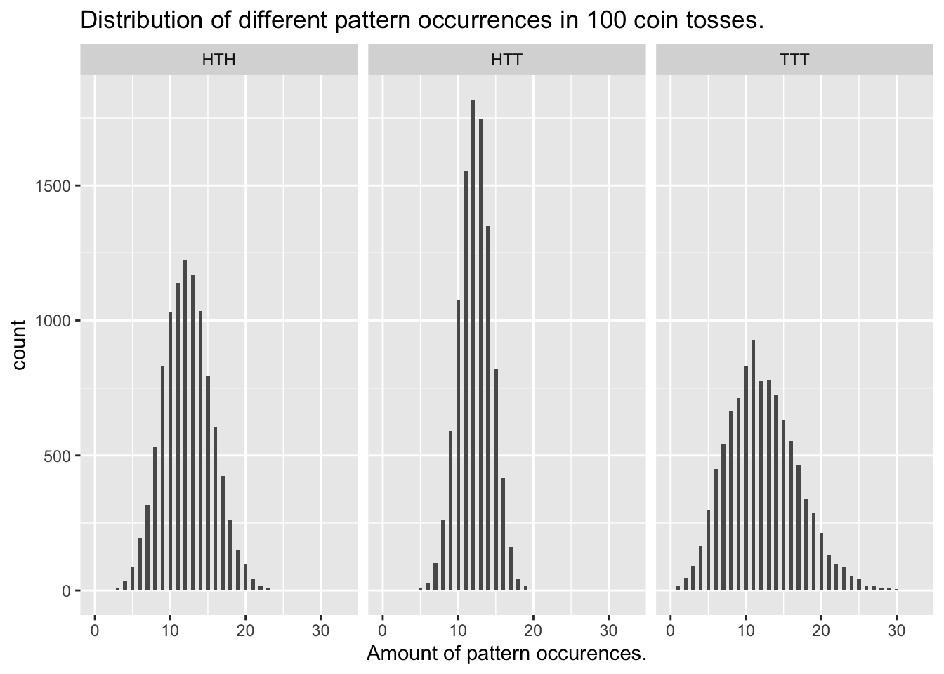

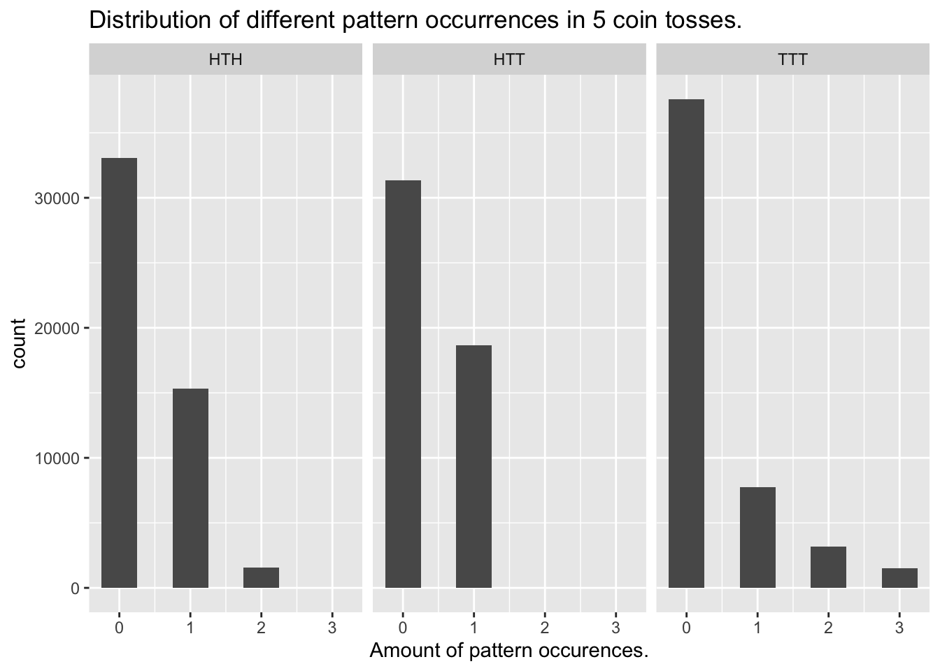
Also interesting: 5 tosses

The means stay the same, but at this few tosses, some patterns can only appear once, while othes (TTT) can appear up to three times when overlapping is allowed.

n_flips =  5

# Running the experiment 10000 times seeking HTH, HTT and TTT
results = data.frame(
  HTH = replicate(50000, count.pattern(HTH, n_flips)),
  HTT = replicate(50000, count.pattern(HTT, n_flips)),
  TTT = replicate(50000, count.pattern(TTT, n_flips))
)
print(summary(results)[4,])

##                HTH                HTT                TTT 
## "Mean   :0.3701  " "Mean   :0.3733  " "Mean   :0.3724  "

ggplot(tidyr::pivot_longer(results,
                           c("HTH", "HTT", "TTT"),
                           names_to = "pattern",
                           values_to = "value"),
       aes(value)) +
  geom_histogram(binwidth = 0.5) +
  facet_wrap(vars(pattern)) +
  labs(x = paste("Amount of pattern occurences.")) +
  ggtitle(paste("Distribution of different pattern occurrences in", n_flips, "coin tosses."))