Gradient Descent overview

Problem: We can estimate the \(\hat{\theta}\) coefficients by minimizing the empirical risk \[ R_{e m p}(f)=\frac{1}{n} \sum_{i=1}^n L\left(y^{(i)}, f\left(x^{(i)} \mid \theta\right)\right) \] of the model over \(\theta\). With quadratic loss, this yields \[ R_{e m p}(f)=\frac{1}{n} \sum_{i=1}^n\left(y^{(t)}-\left(x^{(i)}\right)^T \hat{\theta}\right)^2 \] This can be written in matrix notation as: \[ R_{\mathrm{emp}}(f)=\frac{1}{n}(X \theta-y)^T(X \theta-y)=\frac{1}{n}\left[\theta^T X^T X \theta-2 \theta^T X^T y+y^T y\right] \] and our optimization problem becomes: \[ \hat{\theta}=\arg \min _\theta R_{\mathrm{emp}}(f) \] Solution: - we can solve this kind of minimization problem using an iterative technique termed Gradient Descent - this is an extremely important technique that is applied - in many variants - to solve the optimization problem when optimizing many kinds of learners. - Note: An analytic solution exists for the quadratic loss, s.t. \[ \hat{\theta}=\left(X^T X\right)^{-1} X^T y \] Gradient Descent: The Gradient Descent method follows this algorithm: 0. Initialize \(\theta^{[0]}\) (randomly) and calculate the gradient of the empirical risk with respect to \(\theta\), for example for the squared error loss: \[ \frac{\partial R_{\text {emp }}(f)}{\partial \theta}=\frac{\partial}{\partial \theta}\left(\frac{1}{n}\left[\theta^T X^T X \theta-2 \theta^T X^T y+y^T y\right]\right)=\frac{2}{n} X^T[X \theta-y] \] Now iterate these two steps: 1. Evaluate the gradient at the current value of the parameter vector \(\theta^{[t]}\) : \[ \left.\frac{\partial R_{\mathrm{emp}}(f)}{\partial \theta}\right|_{\theta=\theta^{[t]}}=\frac{2}{n} X^T\left[X \theta^{[t]}-y\right] \] 2. update the estimate for \(\theta\) using this formula: \[ \theta^{[t+1]}=\theta^{[t]}-\left.\lambda \frac{\partial R_{\operatorname{emp}}(f)}{\partial \theta}\right|_{\theta=\theta[t]} \] - The stepsize or learning rate parameter \(\lambda\) controls the size of the updates per iteration \(t\). - We stop if the differences between successive updates of \(\theta\) are below a certain threshold or once a maximum number of iterations is reached. - Many variants of gradient descent exist that either - develop clever ways on how to choose good stepsizes (maybe even dependent on \(t\) ), - and/or how to compute (approximations to) the gradient effectively, - and/or even adapt the direction of the update itself by taking into account, for example, the previously used update directions or the second derivatives of the empirical risk (i.e., the curvature of the risk surface). # Function Definitions ## L2 Risk

# Calculate quadratic risk
# This function calculates the L2 risk of a linear regression model
# Inputs:
# - Y: a numeric vector of response variable
# - X: a matrix of predictor variables
# - theta: a numeric vector of regression coefficients
# Outputs:
# - quadratic_risk: a numeric value representing the L2 risk of the model
calculate_L2_risk <- function(Y, X, theta) {
  squared_diff <- (X %*% theta - Y) ^ 2
  quadratic_risk <- 1 / nrow(X) * sum(squared_diff)
  return(quadratic_risk)
}

calculate_L1_risk <- function(Y, X, theta) {
  mean(abs(X %*% theta - Y))
}

absolute_gradient <- function(Y, X, theta) {
  1 / nrow(X) * t(X) %*% sign(X %*% theta - Y)
}

squared_gradient <- function(Y, X, theta) {
  2 / nrow(X) * (t(X) %*% (X %*% theta - Y))
}

# Y: a vector of response values (dependent variable).
# X: a matrix of predictor values (independent variables).
# theta: a vector of initial coefficients.
# risk: a function that computes the empirical risk given the response Y, predictor X, and coefficients theta. The default is risk_quadratic, which computes the squared error loss.
# gradient: a function that computes the gradient of the empirical risk given the response Y, predictor X, and coefficients theta. The default is gradient_quadratic, which computes the gradient of the squared error loss.
# lambda: a scalar representing the learning rate, which controls the step size for each iteration of gradient descent. The default value is 0.005.
# epsilon: a scalar representing the convergence threshold. The optimization algorithm stops when the change in coefficients between two iterations is less than epsilon. The default value is 0.0001.
# max_iterations: a scalar representing the maximum number of iterations allowed for gradient descent. The default value is 2000.
# min_learning_rate and max_learning_rate: scalar values representing the lower and upper bounds of the learning rate. The default values are 0 and 1000, respectively.
# plot: a boolean indicating whether or not to plot the coefficient values and loss function over iterations. The default value is TRUE.
# include_storage: a boolean indicating whether or not to include the storage of loss and coefficient values in the returned object. The default value is FALSE.

gradient_descent <- function(
    Y, X, theta,
    risk = calculate_L2_risk,
    gradient = squared_gradient,
    lambda = 0.005,
    epsilon = 0.0001,
    max_iterations = 2000,
    min_learning_rate = 0,
    max_learning_rate = 1000,
    plot = TRUE,
    include_storage = FALSE) {
  loss_storage <- data.frame(
    iterations = seq_len(max_iterations) - 1,
    loss = NA
  )
  theta_storage <- matrix(NA, ncol = length(theta), nrow = max_iterations + 1)
  loss_storage[1, "loss"] <- risk(Y, X, theta)
  theta_storage[1, ] <- theta
  
  for (i in 1:max_iterations) {
    grad <- gradient(Y = Y, X = X, theta = theta)
    lambda_opt <- optim(
      par = lambda, # start value
      fn = function(lambda) risk(Y = Y, X = X, theta = theta - lambda * grad), # to min
      method = "Brent", # 1d minimization
      lower = min_learning_rate,
      upper = max_learning_rate,
    )$par
    theta <- theta - lambda_opt * grad
    loss_storage[i + 1, "loss"] <- risk(Y = Y, X = X, theta = theta)
    theta_storage[i + 1, ] <- t(theta)
    
    if (i > 1 && sqrt(sum((theta_storage[i, ] - theta_storage[i + 1, ])^2)) < epsilon) {
      break
    }
  }
  if (plot) {
    layout(t(1:(length(theta) + 1)))
    for (i in 1:length(theta)) {
      plot(
        x = seq_along(theta_storage[, i]) - 1, y = theta_storage[, i],
        ylab = "coefficient value",
        xlab = "iteration", type = "l", col = "blue",
        main = bquote(theta[.(i - 1)])
      )
    }
    plot(
      x = seq_along(loss_storage[, "loss"]) - 1, y = loss_storage[, "loss"],
      ylab = "empirical risk",
      xlab = "iteration", type = "l", col = "red",
      main = expression(R[emp](theta))
    )
  }
  if (include_storage) {
    list(
      theta = theta, risk = risk(Y, X, theta),
      storage = list(loss = loss_storage, theta = theta_storage)
    )
  } else {
    list(theta = theta, risk = risk(Y, X, theta))
  }
}

Put into practice

set.seed(1337)
n <- 500
# design matrix
X <- cbind(
1,
runif(n, -5, 5),
runif(n, -3, 10))

true_theta <- c(2, 0.5, 0.5)
Y <- X %*% true_theta + rnorm(n)

theta_init <- rep(0, ncol(X))
gradient_descent(Y = Y, X = X, theta = theta_init)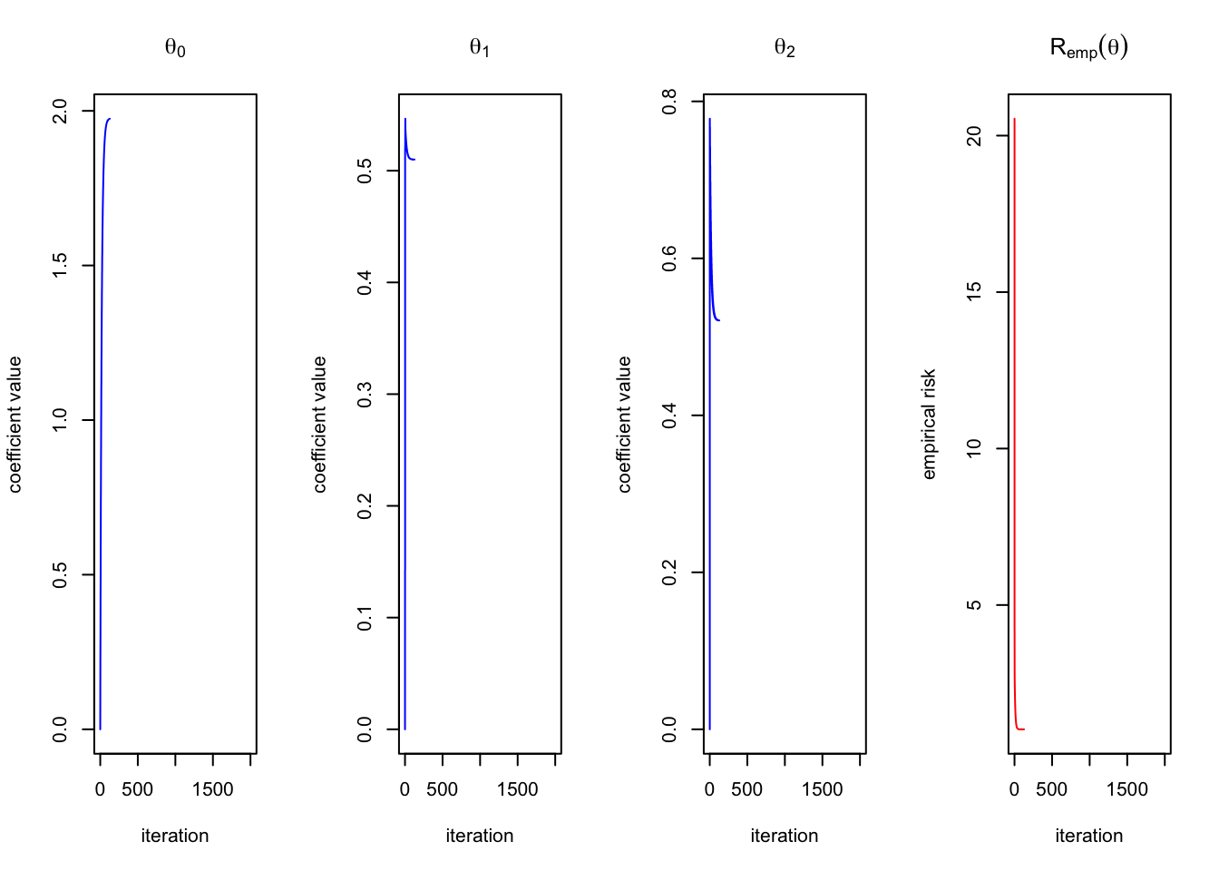

## $theta
##           [,1]
## [1,] 1.9746279
## [2,] 0.5099878
## [3,] 0.5209291
## 
## $risk
## [1] 1.028384

gradient_descent(Y = Y, X= X, theta = theta_init, gradient = absolute_gradient, risk = calculate_L1_risk)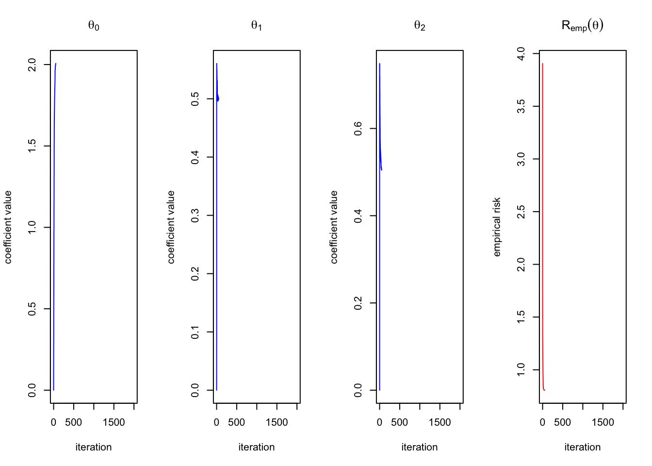

## $theta
##           [,1]
## [1,] 2.0063431
## [2,] 0.4992328
## [3,] 0.5054437
## 
## $risk
## [1] 0.8064193