Introduction

Principal Component Analysis (PCA) is a widely used statistical technique that is used to reduce the dimensionality of large datasets, while still preserving the important information contained within them. The method is particularly useful when dealing with datasets that contain a large number of variables, and the aim is to identify the most important variables that explain the majority of the variation in the data.

In this blog post, we will discuss the theory behind PCA, its use cases, and provide a case study of how to perform PCA in R.

Theory behind PCA

PCA is a mathematical technique that involves transforming a set of correlated variables into a new set of uncorrelated variables, called principal components. The principal components are arranged in order of their variance, with the first principal component having the largest variance, and each subsequent component having progressively smaller variances.

The first principal component is a linear combination of the original variables that explains the most variation in the data. The second principal component is a linear combination of the original variables that explains the second most variation, and so on. The number of principal components is equal to the number of variables in the original dataset.

The transformation is carried out by finding the eigenvectors and eigenvalues of the covariance matrix of the original dataset. The eigenvectors represent the directions in which the data varies the most, while the eigenvalues represent the amount of variation in each direction. By selecting only the eigenvectors corresponding to the largest eigenvalues, we can obtain a smaller set of uncorrelated variables that capture the most important information in the original dataset.

Mathematically, the transformation can be expressed as follows:

Let \(X\) be a \(n \times p\) matrix of \(n\) observations and \(p\) variables. We first standardize the data by subtracting the mean of each variable and dividing by its standard deviation. This ensures that all variables have the same scale.

The covariance matrix of the standardized data is given by:

\[ \boldsymbol{S}=\frac{1}{n-1} X^T X \]

The eigenvectors and eigenvalues of S are then calculated, such that: \[S \mathbf{v}=\lambda \mathbf{v}\]

where \(\textbf{v}\) is the eigenvector and \(\lambda\) is the corresponding eigenvalue.

The principal components are then calculated as:

\[\mathbf{P C}_i=\mathbf{X} \mathbf{v}_i\]

where \(\textbf{PC}_i\) is the ith principal component, \(\textbf{X}\) is the original data matrix, and \(\textbf{v}_i\) is the ith eigenvector.

Use cases

PCA has a wide range of applications in data analysis, including:

• Data compression PCA can be used to reduce the dimensionality of large datasets, making them easier to store and analyze.

• Feature selection: PCA can be used to identify the most important variables in a dataset, which can then be used for further analysis.

• Image processing: PCA can be used to reduce the size of digital images without losing important information.

• Finance: PCA can be used to identify the underlying factors that drive the variation in financial data, such as stock prices or interest rates.

Performing PCA in R

The Swiss dataset is a classical dataset in R that contains information on various aspects of life in the 47 Swiss cantons in 1888. The dataset has 47 observations (one for each canton) and 6 variables, including fertility rate (per capita), agriculture (percentage of males involved in agriculture), examination results (percentage of conscripts with highest mark), education (percentage of education beyond primary school for each canton), Catholic (percentage of Catholics in the population), and infant mortality (number of infant deaths per 1,000 live births). This dataset is often used in statistical education and is useful for demonstrating basic statistical concepts such as regression and PCA.

data(swiss)
str(swiss)

## 'data.frame':    47 obs. of  6 variables:
##  $ Fertility       : num  80.2 83.1 92.5 85.8 76.9 76.1 83.8 92.4 82.4 82.9 ...
##  $ Agriculture     : num  17 45.1 39.7 36.5 43.5 35.3 70.2 67.8 53.3 45.2 ...
##  $ Examination     : int  15 6 5 12 17 9 16 14 12 16 ...
##  $ Education       : int  12 9 5 7 15 7 7 8 7 13 ...
##  $ Catholic        : num  9.96 84.84 93.4 33.77 5.16 ...
##  $ Infant.Mortality: num  22.2 22.2 20.2 20.3 20.6 26.6 23.6 24.9 21 24.4 ...

swiss_data <- swiss[, -1]
swiss_std <- scale(swiss_data)
swiss_pca <- prcomp(swiss_std, center = TRUE, scale. = TRUE)
summary(swiss_pca)

## Importance of components:
##                           PC1    PC2    PC3     PC4     PC5
## Standard deviation     1.6228 1.0355 0.9033 0.55928 0.40675
## Proportion of Variance 0.5267 0.2145 0.1632 0.06256 0.03309
## Cumulative Proportion  0.5267 0.7411 0.9043 0.96691 1.00000

The scree plot will show us the proportion of variance explained by each component graphically. The biplot will show us the relationship between the variables and the principal components.

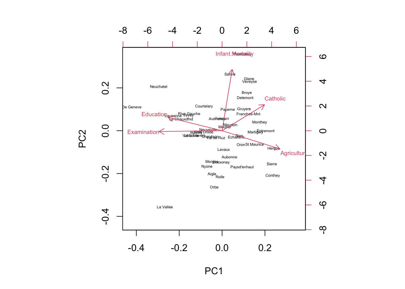
We can see that the first two principal components explain over 70% of the variance in the data. The biplot shows that variables such as fertility rate, percentage of Catholic population, and infant mortality rate are strongly correlated with each other and contribute most to the first principal component, which can be interpreted as a measure of socio-economic development. The second principal component is mainly driven by variables such as agricultural productivity and education level.

plot(swiss_pca, type = "l") #Scree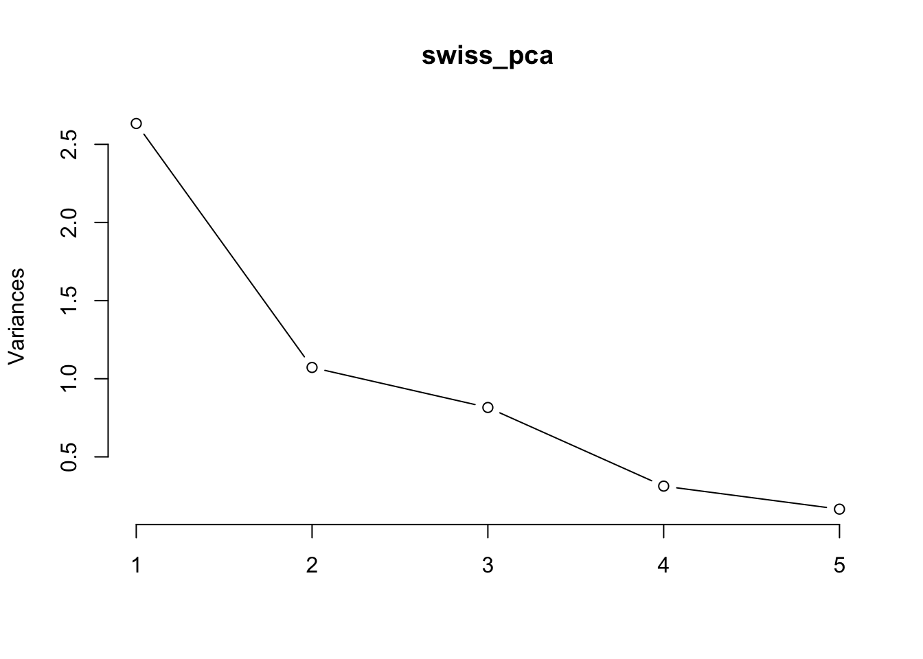 

biplot(swiss_pca, cex=c(0.4,0.6)) # Biplot