Generative Classification Models
Max / 2023-02-15
Generative Classification methods
Theory
When we are using a generative approach to classification, we are not modeling the conditional density \(\pi_k(x) = P(y = k | x)\), i.e., the class membership probability given a certain feature vector, directly. Instead, we are modeling the “other” conditional density \(f(x | y = k)\) (“probability” of a feature vector given a certain class membership, i.e. the likelihood of observing \(x\) under the assumption that the class is \(k\)). Following the Bayes’ rule one gets that
\[ \pi_k(x) \propto \pi_k \cdot f(x | y = k). \] The distribution defined by the parameters \(\pi_k\) is called the prior and can be interpreted as the representation of our a priori knowledge about the frequencies of the target classes. In our setting we can use a straightforward approach to deriving this prior, s.t.
\[ \hat{\pi}_k = \frac{n_k}{n}. \] With prior and likelihood specified, we can use the fact that all posterior class probabilities need to sum to one to get: \[ 1 = \sum^{g}_{j=1} \pi_j(x) = \sum^{g}_{j=1}\alpha \pi_j \cdot p(x | y = j) \iff \alpha = \frac{1}{\sum^{g}_{j=1}\pi_j \cdot p (x | y = j)}. \] From this, we see that \(\pi_k(x)\) can be expressed as \[ \pi_k(x) = \frac{\pi_k \cdot p(x | y = k)}{\sum^{g}_{j=1}\pi_j \cdot p(x | y = j)}. \]
Data
In this code demo we’re looking at the iris data set again:
library(ggplot2)
data(iris)
target <- "Species"
features <- c("Sepal.Width", "Sepal.Length")
iris_train <- iris[, c(target, features)]
target_levels <- levels(iris_train[, target])
ggplot(iris_train, aes(x = Sepal.Width, y = Sepal.Length)) +
  geom_point(aes(color = Species))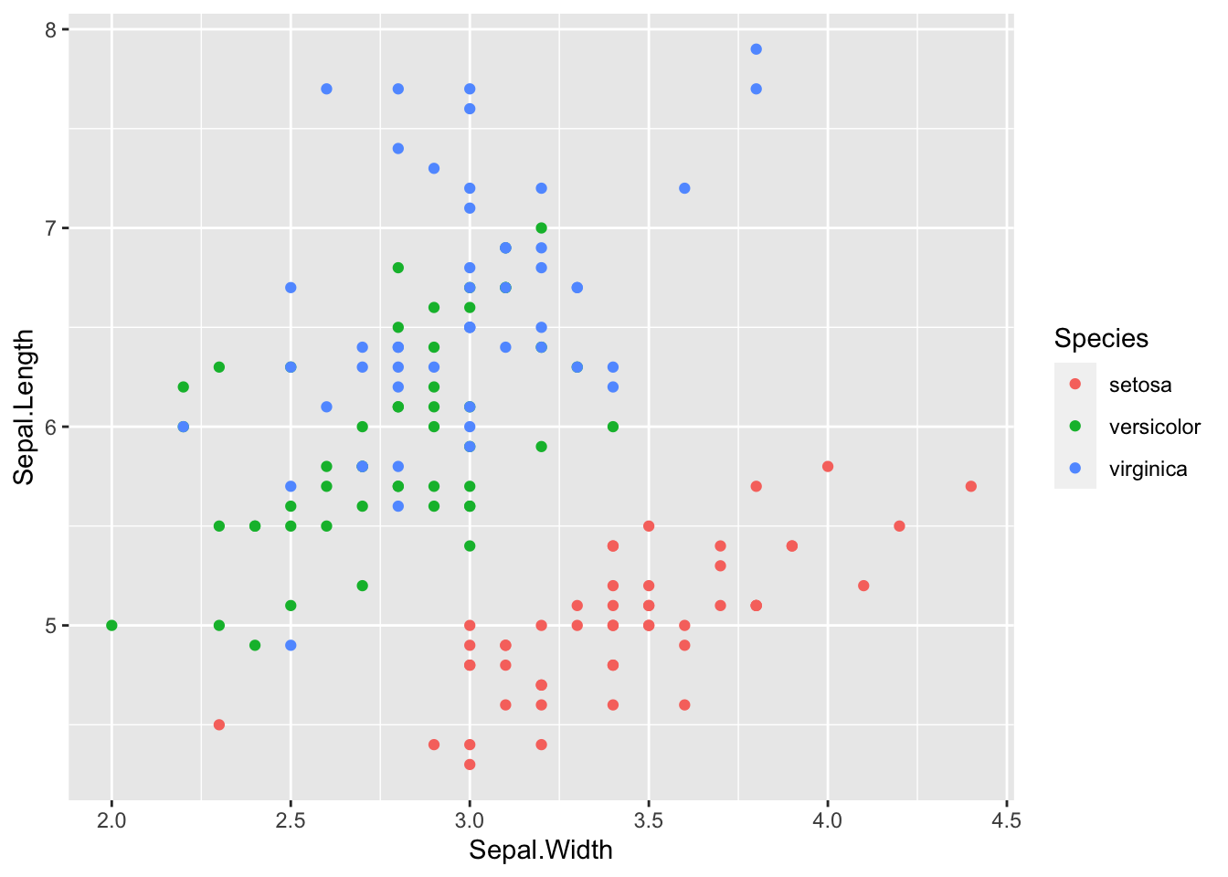
For the estimation of the models we will mostly use the mlr3-package, s.t.
we firstly have to define a task:
library(mlr3)
library(mlr3learners)
iris_task <- TaskClassif$new(id = "iris_train", backend = iris_train,
                             target = target)
Models (& More Theory)
Linear discriminant analysis (LDA)
In LDA, we model the likelihood as a multivariate normal distribution s.t. \[ p(x | y = k) = \frac{1}{\pi^{\frac{p}{2}} |\Sigma|^{\frac{1}{2}}}\exp\left(- \frac{1}{2} (x-\mu_k)^T\Sigma^{-1}(x-\mu_k)\right). \] With:
- \(\hat{\mu}_k = \frac{1}{n_k}\sum_{i: y^{(i)} = k} x^{(i)},\)
- \(\hat{\Sigma} = \frac{1}{n - g} \sum_{k=1}^g\sum_{i: y^{(i)} = k} (x^{(i)} - \hat{\mu}_k)(x^{(i)} - \hat{\mu}_k)^T.\)
For every class, it is assumed that data is normally distributed with the same covariance matrix \(\Sigma\) for all classes but different mean vectors \(\mu_k\).
We train the model:
iris_lda_learner <- lrn("classif.lda", predict_type = "prob")
iris_lda_learner$train(task = iris_task)
We create a general framework for likelihoods, s.t. the we are able to visualize them:
library(mvtnorm)

get_mvgaussian_lda <- function(data, target, level, features) {
  classif_task <- TaskClassif$new(id = "mvg_task",
    backend = data[, c(features, target)],
    target = target
  )
  lda_learner <- lrn("classif.lda")
  lda_learner$train(task = classif_task)

  list(
    mean = lda_learner$model$means[level, features],
    sigma = solve(tcrossprod(lda_learner$model$scaling[features, ])),
    type = "mv_gaussian",
    features = features
  )
}


likelihood <- function(likelihood_def, data) {
  switch(likelihood_def$type,
    mvgaussian_lda = get_mvgaussian_lda(
      data, likelihood_def$target,
      likelihood_def$level,
      likelihood_def$features
    )
  )
}
predict_likelihood <- function(likelihood, x) {
  switch(likelihood$type,
    mv_gaussian = dmvnorm(x,
      mean = likelihood$mean,
      sigma = likelihood$sigma
    )
  )
}
We write a plot function for multivariate likelihood functions with two features:
library(reshape2)

plot_2D_likelihood <- function(likelihoods, data, X1, X2, target, lengthX1 = 100,
                               lengthX2 = 100) {
  gridX1 <- seq(
    min(data[, X1]),
    max(data[, X1]),
    length.out = lengthX1
  )
  gridX2 <- seq(
    min(data[, X2]),
    max(data[, X2]),
    length.out = lengthX2
  )
  grid_data <- expand.grid(gridX1, gridX2)
  features <- c(X1, X2)
  target_levels <- names(likelihoods)
  names(grid_data) <- features
  lik <- sapply(target_levels, function(level) {
    likelihood <- likelihoods[[level]]
    predict_likelihood(likelihood, grid_data[, likelihood$features])
  })
  grid_data <- cbind(grid_data, lik)
  to_plot <- melt(grid_data, id.vars = features)
  ggplot() +
    geom_contour(
      data = to_plot,
      aes_string(x = X1, y = X2, z = "value", color = "variable")
    ) +
    geom_point(data = data, aes_string(x = X1, y = X2, color = target))
}
lda_liks <- sapply(target_levels, function(level)
likelihood(
likelihood_def = list(
type = "mvgaussian_lda", target = target,
level = level, features = features
),
iris_train
),
simplify = FALSE
)
plot_2D_likelihood(lda_liks, iris_train, "Sepal.Width", "Sepal.Length", target)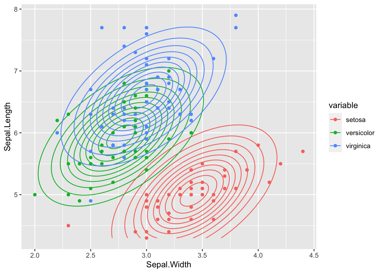
We clearly see that all class distributions are modeled with the same covariance matrix - the shape and orientation of the contour lines of all 3 class distributions is the same.
library(mlr3viz)
plot_learner_prediction(iris_lda_learner, iris_task) +
  guides(alpha = "none", shape = "none")
## INFO [17:50:28.779] [mlr3] Applying learner 'classif.lda' on task 'iris_train' (iter 1/1)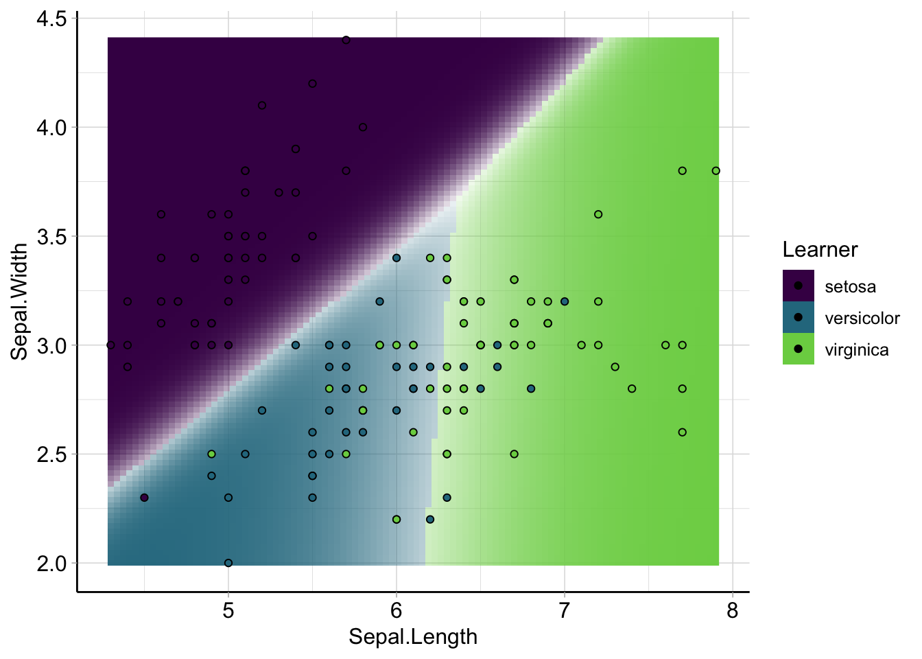 The resulting decision boundaries are linear – even though we can’t really clearly see that in the contour plot above.
Quadratic discriminant analysis (QDA)
In QDA, we model the likelihood as a multivariate normal distribution s.t. \[ p(x | y = k) = \frac{1}{\pi^{\frac{p}{2}} |\Sigma_k|^{\frac{1}{2}}}\exp\left(- \frac{1}{2} (x-\mu_k)^T\Sigma_k^{-1}(x-\mu_k)\right) \] With:
- \(\hat{\mu}_k = \frac{1}{n_k}\sum_{i: y^{(i)} = k} x^{(i)},\)
- \(\hat{\Sigma}_k = \frac{1}{n_k - 1} \sum_{i: y^{(i)} = k} (x^{(i)} - \hat{\mu}_k)(x^{(i)} - \hat{\mu}_k)^T.\)
This means we estimate a different mean vector and covariance matrix for for every class.
iris_qda_learner <- lrn("classif.qda", predict_type = "prob")
iris_qda_learner$train(task = iris_task)
We define all we need for our likelihood framework and plot them:
get_mvgaussian_qda <- function(data, target, level, features) {
  classif_task <- TaskClassif$new(id = "mvg_task",
    backend = data[, c(features, target)],
    target = target
  )
  qda_learner <- lrn("classif.qda")
  qda_learner$train(task = classif_task)

  list(
    mean = qda_learner$model$means[level, features],
    sigma = solve(tcrossprod(qda_learner$model$scaling[features, ,
                                                             level])),
    type = "mv_gaussian",
    features = features
  )
}
likelihood <- function(likelihood_def, data) {
  switch(likelihood_def$type,
    mvgaussian_lda = get_mvgaussian_lda(
      data, likelihood_def$target,
      likelihood_def$level,
      likelihood_def$features
    ),
    mvgaussian_qda = get_mvgaussian_qda(
      data, likelihood_def$target,
      likelihood_def$level,
      likelihood_def$features
    )
  )
}
liks <- sapply(target_levels, function(level)
  likelihood(list(
    type = "mvgaussian_qda", target = target,
    level = level, features = features
  ), iris_train), simplify = FALSE)
plot_2D_likelihood(liks, iris_train, "Sepal.Width", "Sepal.Length", target)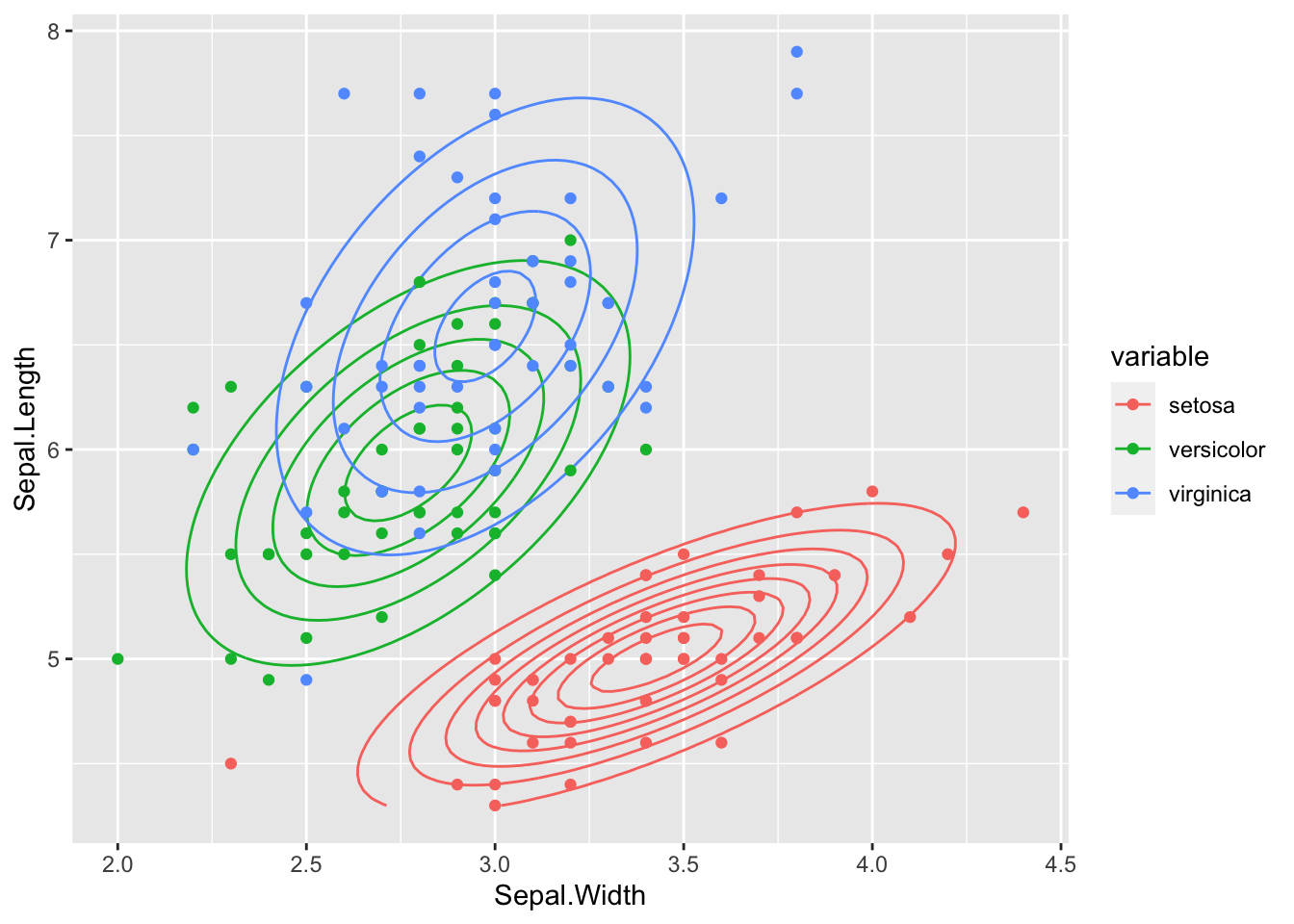
As we can see, the covariance is now different in each class.